VLIZ |
|
Flanders Marine Institute (VLIZ) - Geoserver WMS Service
| Service health Now: |
|---|
- Interface
- Web Service, OGC Web Map Service 1.3.0
- Keywords
- WFS, WMS, GEOSERVER
- Fees
- NONE
- Access constraints
- Please contact VLIZ if you want to use a layer
- Supported languages
- No INSPIRE Extended Capabilities (including service language support) given. See INSPIRE Technical Guidance - View Services for more information.
- Data provider
-
VLIZ (unverified)
Contact information:
Flanders Marine Institute
VLIZ
Work:
Ostend, BelgiumEmail:
- Service metadata
- No INSPIRE Extended Capabilities (including service metadata) given. See INSPIRE Technical Guidance - View Services for more information.
Ads by Google
A compliant implementation of OGC WMS.
Available map layers (1131)
EMODnet EurOBIS Occurences as Geospatial Grid (Dataportal:eurobis_rasters-obisenv)
The Occurences as Geospatial Grid summarises occurences as the number of occurences in a geospatial grid. There are four grid size levels available, plus the possibility of retrieving each point directly. For more information, please consult: https://github.com/EMODnet/EMODnet-Biology-Guidance.
Bodemtextuur (ecosysteemdiensten:Bodemtextuur)
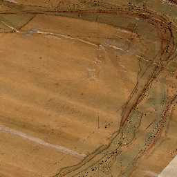
Topografische kaart van de regio rond Aalst, gemaakt door Depot de la Guerre, 1893 (HistorischeKaarten:DepotDeLaGuerre_Aalst_1893)
Topografische kaart van de regio rond Aalst, gemaakt door Depot de la Guerre, 1929 (HistorischeKaarten:DepotDeLaGuerre_Aalst_1929)
Topografische kaart van de Schelde nabij Antwerpen, gemaakt door Depot de la Guerre, 1892 (HistorischeKaarten:DepotDeLaGuerre_Antwerpen_1892)
Topografische kaart van de Schelde nabij Antwerpen, gemaakt door Depot de la Guerre, 1903 (HistorischeKaarten:DepotDeLaGuerre_Antwerpen_1902)
Topografische kaart van de Schelde nabij Appels, gemaakt door Depot de la Guerre, 1893 (HistorischeKaarten:DepotDeLaGuerre_Appels_1893)
Topografische kaart van de Schelde nabij Appels, gemaakt door Depot de la Guerre, 1910 (HistorischeKaarten:DepotDeLaGuerre_Appels_1910)
Topografische kaart van de Schelde nabij Berendrecht, gemaakt door Depot de la Guerre, 1892 (HistorischeKaarten:DepotDeLaGuerre_Berendrecht_1892)
Topografische kaart van de Schelde nabij Berendrecht, gemaakt door Depot de la Guerre, 1933 (HistorischeKaarten:DepotDeLaGuerre_Berendrecht_1933)
Topografische kaart van de Rupel nabij Boom, gemaakt door Depot de la Guerre, 1892 (HistorischeKaarten:DepotDeLaGuerre_Boom_1892)
Topografische kaart van de Rupel nabij Boom, gemaakt door Depot de la Guerre, 1930 (HistorischeKaarten:DepotDeLaGuerre_Boom_1930)
Topografische kaart van de Schelde nabij Dendermonde, gemaakt door Depot de la Guerre, 1893 (HistorischeKaarten:DepotDeLaGuerre_Dendermonde_1893)
Topografische kaart van de Schelde nabij Dendermonde, gemaakt door Depot de la Guerre, 1930 (HistorischeKaarten:DepotDeLaGuerre_Dendermonde_1930)
Topografische kaart van de Schelde nabij Destelbergen, gemaakt door Depot de la Guerre, 1893 (HistorischeKaarten:DepotDeLaGuerre_Destelbergen_1893)
Topografische kaart van de Schelde nabij Destelbergen, gemaakt door Depot de la Guerre, 1910 (HistorischeKaarten:DepotDeLaGuerre_Destelbergen_1910)
Topografische kaart van de Schelde nabij Doel, gemaakt door Depot de la Guerre, 1892 (HistorischeKaarten:DepotDeLaGuerre_Doel_1892)
Topografische kaart van de Schelde nabij Doel, gemaakt door Depot de la Guerre, 1928 (HistorischeKaarten:DepotDeLaGuerre_Doel_1928)
Topografische kaart van de Schelde nabij Hemixem, gemaakt door Depot de la Guerre, 1892 (HistorischeKaarten:DepotDeLaGuerre_Hemixem_1892)
Topografische kaart van de regio rond Hemixem, gemaakt door Depot de la Guerre, 1922 (HistorischeKaarten:DepotDeLaGuerre_Hemixem_1922)
Topografische kaart van de Schelde nabij Kallo, gemaakt door Depot de la Guerre, 1892 (HistorischeKaarten:DepotDeLaGuerre_Kallo_1892)
Topografische kaart van de Schelde nabij Kallo, gemaakt door Depot de la Guerre, 1903 (HistorischeKaarten:DepotDeLaGuerre_Kallo_1903)
Topografische kaart van de regio nabij Lokeren, gemaakt door Depot de la Guerre, 1893 (HistorischeKaarten:DepotDeLaGuerre_Lokeren_1893)
Topografische kaart van de regio rond Lokeren, gemaakt door Depot de la Guerre, 1910 (HistorischeKaarten:DepotDeLaGuerre_Lokeren_1910)
Topografische kaart van de Schelde nabij de NoordlandPolder, gemaakt door Depot de la Guerre, 1881 (HistorischeKaarten:DepotDeLaGuerre_NoordlandPolder_1881)
Topografische kaart van de Schelde nabij de NoordlandPolder, gemaakt door Depot de la Guerre, 1928 (HistorischeKaarten:DepotDeLaGuerre_NoordlandPolder_1928)
Topografische kaart van de Schelde nabij Oordegem, gemaakt door Depot de la Guerre, 1893 (HistorischeKaarten:DepotDeLaGuerre_Oordegem_1893)
Topografische kaart van de regio rond Oordegem, gemaakt door Depot de la Guerre, 1910 (HistorischeKaarten:DepotDeLaGuerre_Oordegem_1910)
Topografische kaart van de regio rond Oosterzele, gemaakt door Depot de la Guerre, 1893 (HistorischeKaarten:DepotDeLaGuerre_Oosterzele_1893)
Topografische kaart van de regio nabij Oosterzele, gemaakt door Depot de la Guerre, 1910 (HistorischeKaarten:DepotDeLaGuerre_Oosterzele_1910)
Topografische kaart van de Schelde nabij St Amands, gemaakt door Depot de la Guerre, 1892 (HistorischeKaarten:DepotDeLaGuerre_StAmands_1892)
Topografische kaart van de Schelde nabij St Amands, gemaakt door Depot de la Guerre, 1930 (HistorischeKaarten:DepotDeLaGuerre_StAmands_1930)
Topografische kaart van de regio rond St Niklaas, gemaakt door Depot de la Guerre, 1892 (HistorischeKaarten:DepotDeLaGuerre_StNiklaas_1892)
Topografische kaart van de regio rond St Niklaas, gemaakt door Depot de la Guerre, 1909 (HistorischeKaarten:DepotDeLaGuerre_StNiklaas_1909)
Topografische kaart van de Schelde nabij Temse, gemaakt door Depot de la Guerre, 1892 (HistorischeKaarten:DepotDeLaGuerre_Temse_1892)
Topografische kaart van de Schelde nabij Temse, gemaakt door Depot de la Guerre, 1903 (HistorischeKaarten:DepotDeLaGuerre_Temse_1903)
Topografische kaart van de Schelde nabij Uitbergen, gemaakt door Depot de la Guerre, 1893 (HistorischeKaarten:DepotDeLaGuerre_Uitbergen_1893)
Topografische kaart van de Schelde nabij Uitbergen, gemaakt door Depot de la Guerre, 1910 (HistorischeKaarten:DepotDeLaGuerre_Uitbergen_1910)
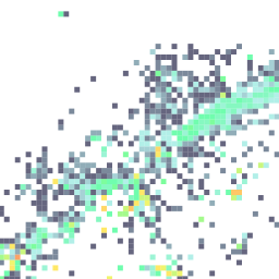
EMOD-PACE - WP5 Vessel traffic density - Other (EMODPACE:EMOD-PACE_VD_2019_01_st_00)
EMOD-PACE - WP5 Vessel traffic density - Fishing (EMODPACE:EMOD-PACE_VD_2019_01_st_01)
EMOD-PACE - WP5 Vessel traffic density - Service (EMODPACE:EMOD-PACE_VD_2019_01_st_02)
EMOD-PACE - WP5 Vessel traffic density - Dredging or underwater ops (EMODPACE:EMOD-PACE_VD_2019_01_st_03)
EMOD-PACE - WP5 Vessel traffic density - Sailing (EMODPACE:EMOD-PACE_VD_2019_01_st_04)
EMOD-PACE - WP5 Vessel traffic density - Pleasure craft (EMODPACE:EMOD-PACE_VD_2019_01_st_05)
EMOD-PACE - WP5 Vessel traffic density - High Speed Craft (EMODPACE:EMOD-PACE_VD_2019_01_st_06)
EMOD-PACE - WP5 Vessel traffic density - Tug and towing (EMODPACE:EMOD-PACE_VD_2019_01_st_07)
EMOD-PACE - WP5 Vessel traffic density - Passenger (EMODPACE:EMOD-PACE_VD_2019_01_st_08)
EMOD-PACE - WP5 Vessel traffic density - Cargo (EMODPACE:EMOD-PACE_VD_2019_01_st_09)
EMOD-PACE - WP5 Vessel traffic density - Tanker (EMODPACE:EMOD-PACE_VD_2019_01_st_10)
EMOD-PACE - WP5 Vessel traffic density - Military and low enforcement (EMODPACE:EMOD-PACE_VD_2019_01_st_11)
EMOD-PACE - WP5 Vessel traffic density - Unknown (EMODPACE:EMOD-PACE_VD_2019_01_st_12)
EMOD-PACE - WP5 Vessel traffic density - All (EMODPACE:EMOD-PACE_VD_2019_01_st_All)
EMOD-PACE - WP5 Vessel traffic density - All (EMODPACE:EMODPACE-VD-2019-All)
EMOD-PACE - WP5 Vessel traffic density - All
EMOD-PACE - WP5 Vessel traffic density - Cargo (EMODPACE:EMODPACE-VD-2019-Cargo)
EMOD-PACE - WP5 Vessel traffic density - Cargo
EMOD-PACE - WP5 Vessel traffic density - Dredging or underwater ops (EMODPACE:EMODPACE-VD-2019-Dredging)
EMOD-PACE - WP5 Vessel traffic density - Dredging or underwater ops
EMOD-PACE - WP5 Vessel traffic density - Fishing (EMODPACE:EMODPACE-VD-2019-Fishing)
EMOD-PACE - WP5 Vessel traffic density - Fishing
EMOD-PACE - WP5 Vessel traffic density - High Speed Craft (EMODPACE:EMODPACE-VD-2019-Highspeed)
EMOD-PACE - WP5 Vessel traffic density - High Speed Craft
EMOD-PACE - WP5 Vessel traffic density - Military and law enforcement (EMODPACE:EMODPACE-VD-2019-Military)
EMOD-PACE - WP5 Vessel traffic density - Military and low enforcement
EMOD-PACE - WP5 Vessel traffic density - Other (EMODPACE:EMODPACE-VD-2019-Other)
EMOD-PACE - WP5 Vessel traffic density - Passenger (EMODPACE:EMODPACE-VD-2019-Passenger)
EMOD-PACE - WP5 Vessel traffic density - Passenger
EMOD-PACE - WP5 Vessel traffic density - Pleasure craft (EMODPACE:EMODPACE-VD-2019-Pleasure)
EMOD-PACE - WP5 Vessel traffic density - Pleasure craft
EMOD-PACE - WP5 Vessel traffic density - Sailing (EMODPACE:EMODPACE-VD-2019-Sailing)
EMOD-PACE - WP5 Vessel traffic density - Sailing
EMOD-PACE - WP5 Vessel traffic density - Service (EMODPACE:EMODPACE-VD-2019-Service)
EMOD-PACE - WP5 Vessel traffic density - Tanker (EMODPACE:EMODPACE-VD-2019-Tanker)
EMOD-PACE - WP5 Vessel traffic density - Tanker
EMOD-PACE - WP5 Vessel traffic density - Tug and towing (EMODPACE:EMODPACE-VD-2019-Tug)
EMOD-PACE - WP5 Vessel traffic density - Tug and towing
EMOD-PACE - WP5 Vessel traffic density - Unknown (EMODPACE:EMODPACE-VD-2019-Unknown)
EMOD-PACE - WP5 Vessel traffic density - Unknown
ETOPO1 global relief model (bedrock) (MarineRegions:ETOPO1_Bed_g_geotiff)
ETOPO1 is a 1 arc-minute global relief model of Earth's surface that integrates land topography and ocean bathymetry. Built from global and regional data sets, it is available in "Ice Surface" (top of Antarctic and Greenland ice sheets) and "Bedrock" (base of the ice sheets). The grid-registered is the authoritative registration. Horizontal datum: WGS 84 geographic Vertical datum: sea level. More specific vertical datums, such as mean sea level, mean high water, and mean low water, differ by less than the vertical accuracy of ETOPO1 (~10 meters at best), and are therefore effectively equivalent.
ETOPO1 global relief model (ice surface) (MarineRegions:ETOPO1_Ice_g_geotiff)
ETOPO1 is a 1 arc-minute global relief model of Earth's surface that integrates land topography and ocean bathymetry. Built from global and regional data sets, it is available in "Ice Surface" (top of Antarctic and Greenland ice sheets) and "Bedrock" (base of the ice sheets). The grid-registered is the authoritative registration. Horizontal datum: WGS 84 geographic
Gemiddelde hoogste grondwaterstand (cm onder maaiveld) (ecosysteemdiensten:Grondwater_ghg_cm)
Gemiddelde hoogste grondwaterstand (cm onder maaiveld)
Gemiddelde laagste grondwaterstand (cm onder maaiveld) (ecosysteemdiensten:Grondwater_glg_cm)
Gemiddelde laagste grondwaterstand (cm onder maaiveld)
Flandria Borealis (HistorischeKaarten:K2_23_2007_271)
Map made by Quad von Kinckelbach, Matthias (graveur); Hogenberg, Frans in the 17° century. More information through the metadata and on the website of HisGISKust.
Copie van een Lant-Caerte der gelegentheit van Vlaanderen en Zeelant ten tyde van Guido van Dampier Grave van Vlaanderen Anno MCCLXXIV. (HistorischeKaarten:K2_25_2007_273)
Map made by Van Thuyne, Lieven in the 18° century. More information through the metadata and on the website of HisGISKust.
Flandria (HistorischeKaarten:K3_10_2007_411)
Map made by Mercator, Gerardus; Ortelius, Abraham in the 16° century. More information through the metadata and on the website of HisGISSchelde.
Exactissima Flandriae descriptio (HistorischeKaarten:K3_20_2007_417)
Map made by de Jode, Cornelis in the 16° century. More information through the metadata and on the website of HisGISKust.
Flandria comit(atus) (HistorischeKaarten:K3_27_2007_420)
Map made by Mercator, Gerardus in the 17° century. More information through the metadata and on the website of HisGISKust.
Beschrijvinghe vande Zeeusche Eijlanden Soe die op hare Stromen geleghen zijn, met een deel vande Zee Custen van Vlaenderen ende hollant. Insularum Zelandiae, partisque Flandriae et Hollandiae accuratissima littoralis descriptio (HistorischeKaarten:K3_41_2007_436)
Map made by Waghenaer, Lucas Jansz in the 16° century. More information through the metadata and on the website of HisGISKust.
Flandria (HistorischeKaarten:K3_45_2007_437)
Map made by Van Berckenrode; Balthasars, Floris in the 17° century. More information through the metadata and on the website of HisGISKust.
Flandria (HistorischeKaarten:K3_45_2007_437_3)
Kaart gemaakt door Van Berckenrode; Balthasars, Floris (1603)
Celeberrimi Flandriae comitatus typus (HistorischeKaarten:K3_52_2007_462)
Map made by Kaerius, Petrus in the 17° century. More information through the metadata and on the website of HisGISSchelde.
Flandriae pars orientalior (HistorischeKaarten:K3_53_2007_461)
Map made by Kaerius, Petrus in the 17° century. More information through the metadata and on the website of HisGISKust.
Kaerte van Sluys, het Zwin, ende de schansen aen weder syden (HistorischeKaarten:K3_59_2007_464)
Map made by in the 17° century. More information through the metadata and on the website of HisGISKust.
Caerte van t'Vrye sijnde een gedeelte en lidt van Vlaenderen waer in vertoont wert de tegenwoordige ghelegentheijt van de stadt Sluys Cadsand en de doorgesteken polders met grooten vlijt gecorrigeert en verbetert (HistorischeKaarten:K3_60_2007_465)
Map made by Visscher, Claes Jansz; Hondius, Henricus (graveur) in the 17° century. More information through the metadata and on the website of HisGISKust.
Caerte van t'Vrye synde een gedeelte van Vlaendren van nieus gecorigeert en met vlijt gebetert (HistorischeKaarten:K3_61_2007_466)
Map made by Visscher, Claes Jansz in the 17° century. More information through the metadata and on the website of HisGISKust.
Comitatus Flandriae nova tabula (HistorischeKaarten:K3_65_2007_467)
Map made by Hondius, Henricus; Hondius, Joannes in the 17° century. More information through the metadata and on the website of HisGISKust.
Pars Flandriae orientalis; Franconatum, insulam Cadsant etc. Civitatesque Gandavum,Brugas, Slusam, Oostendam aliasque continens (HistorischeKaarten:K3_66_2007_468)
Map made by Hondius, Henricus in the 17° century. More information through the metadata and on the website of HisGISKust.
Pascaert vande Custe van Vlaenderen, van Walcheren tot Cales en Boulogne in Vranckrijck (HistorischeKaarten:K3_67_2007_469)
Map made by Hondius, Henricus; Codde, Pieter (tekenaar) in the 17° century. More information through the metadata and on the website of HisGISKust.
Flandria nova descriptio (HistorischeKaarten:K3_70_2007_470)
Map made by Janssonius, Joannes in the 17° century. More information through the metadata and on the website of HisGISKust.
Castellania Furnensis (HistorischeKaarten:K4_10_2007_507)
Map made by in the 17° century. More information through the metadata and on the website of HisGISKust.
Flandriae partes duae quarum altera proprietaria altera imperialis vulgo dicitur (HistorischeKaarten:K4_12_2007_509)
Map made by Blaeu, Willem Jansz; Blaeu, Joannes in the 17° century. More information through the metadata and on the website of HisGISKust.
Territorium Bergense (HistorischeKaarten:K4_13_2007_510)
Map made by Blaeu, Willem Jansz; Blaeu, Joannes in the 17° century. More information through the metadata and on the website of HisGISKust.
Tabula castelli ad Sandflitam, qua simul inundati agri, alluviones, fossae, alvei, quae Bergas ad Zomam et Antverpiam interjacent, annotantur (HistorischeKaarten:K4_16_2007_513)
Within the HisGISKust initiative, a cooperation agreement was concluded between the Flanders Marine Institute (VLIZ) and the Culture Library (Bruges). Historical maps were selected from the Culture Library collection containing specific information about the coastal zone (dunes, dykes, etc.), the Scheldt estuary and/or the Belgian part of the North Sea (BNZ) (sandbanks, indication bathymetry, etc .). The maps were digitised and georeferenced by VLIZ in order to offer them, together with the necessary metadata in open access, to end users. Shapefiles (eg coastline, dune areas, etc.) based on the georeferened maps are also generated and made freely available.
Novus XVII Inferioris Germaniae Provinciarum Typus de integro multis in locis emendatus (HistorischeKaarten:K4_1_2007_498)
Map made by Blaeu, Willem Jansz in the 17° century. More information through the metadata and on the website of HisGISKust.
Flandria et Zeelandia comitatus (HistorischeKaarten:K4_2_2007_499)
Map made by Blaeu, Willem Jansz; Blaeu, Joannes in the 17° century. More information through the metadata and on the website of HisGISKust.
Episcopatus Gandavensis (HistorischeKaarten:K4_32_2007_539)
Map made by Blaeu, Joannes; Blaeu, Cornelius in the 17° century. More information through the metadata and on the website of HisGISKust.
Flandriae Teutonicae pars orientalior (HistorischeKaarten:K4_3_2007_500)
Map made by Blaeu, Willem Jansz; Blaeu, Joannes in the 17° century. More information through the metadata and on the website of HisGISKust.
Pars Flandriae Teutonicae occidentalior (HistorischeKaarten:K4_4_2007_501)
Map made by Blaeu, Willem Jansz; Blaeu, Joannes in the 17° century. More information through the metadata and on the website of HisGISKust.
Westcappelle (HistorischeKaarten:K4_68_2007_606)
Map made by De Lahoese, J.B. (graveur); Mestdagh, J. (graveur); Ongers, J. (graveur) in the 19° century. More information through the metadata and on the website of HisGISKust.
Episcopatus Brugensis (HistorischeKaarten:K4_6_2007_503)
Map made by Blaeu, Joannes; Blaeu, Cornelius in the 17° century. More information through the metadata and on the website of HisGISKust.
Iprensis episcopatus (HistorischeKaarten:K4_8_2007_505)
Map made by Blaeu, Joannes; Blaeu, Cornelis in the 17° century. More information through the metadata and on the website of HisGISKust.
Duynkercka (HistorischeKaarten:K5_17_2007_1255)
Plan de la ville de Dunkerque et de ses attaques avec les retranchements des Espagnols faicts en l'an 1648 (HistorischeKaarten:K5_19_2007_1257)
Map made by Blaeu, Joannes; du Plovich, Vedastus in the 17° century. More information through the metadata and on the website of HisGISKust.
Gravelinga gallis Gravelines dicta (HistorischeKaarten:K5_23_2007_1261)
Map made by Blaeu, Joannes in the 17° century. More information through the metadata and on the website of HisGISKust.
K5_42_2007_1517 (HistorischeKaarten:K5_42_2007_1517)
Slusa Teutonica Flandriae opp. admodum elegans (HistorischeKaarten:K5_55_2007_1524)
Map made by Janssonius, Joannes; Hogenberg, Frans in the 17° century. More information through the metadata and on the website of HisGISKust.
Nieuwe pascaert bevattende in sich de kust van Vlaenderen vande Wielingen tot de Hoofden (HistorischeKaarten:K6_100_2007_2644)
Map made by van Keulen, Johannes in the 17° century. More information through the metadata and on the website of HisGISKust.
Flandriae pars occidentalis (HistorischeKaarten:K6_106_2007_2903)
Map made by Schenk, Pieter in the 17° century. More information through the metadata and on the website of HisGISKust.
Carte du Comté de Flandre. Dressée sur differens morceaux levez sur les lieux fixez par les observations astronomiques (HistorischeKaarten:K6_111_2007_2918)
Map made by de l' Isle, Guillaume in the 18° century. More information through the metadata and on the website of HisGISKust.
Caarte van t' Graafschap Vlaanderen opgestelt na verscheyde stukken op de plaatsen geteekent en door sterrekundige waarnemingen bevestigt = Carte du Comté de Flandre… (HistorischeKaarten:K6_112_2007_2919)
Map made by de l' Isle, Guillaume in the 18° century. More information through the metadata and on the website of HisGISSchelde.
Nouvelle carte de la province de Flandre (HistorischeKaarten:K6_130_2007_2924)
Map made by Walch, Jean in the 18° century. More information through the metadata and on the website of HisGISKust.
Le Comté de Flandres divisés en ses chastellenies, balliages etc (A) (HistorischeKaarten:K6_15_2007_1892A)
Map made by Jaillot, Hubert in the 18° century. More information through the metadata and on the website of HisGISKust.
Le Comté de Flandres divisés en ses chastellenies, balliages etc (B) (HistorischeKaarten:K6_15_2007_1892B)
Map made by Jaillot, Hubert in the 18° century. More information through the metadata and on the website of HisGISKust.
Comitatus Flandriae tam orientalis quam occidentalis ad usum serenissimi Burgundiae ducis (HistorischeKaarten:K6_16_2007_2124)
Map made by Jaillot, Hubert in the 18° century. More information through the metadata and on the website of HisGISKust.
Comitatus Flandriae nova tabula (HistorischeKaarten:K6_1_2007_1883)
Map made by Mariette, Pierre in the 17° century. More information through the metadata and on the website of HisGISKust.
Fiandra parte occidentale. Zelanda e parte orientale della Fiandra (A) (HistorischeKaarten:K6_25_2007_1882A)
Map made by Coronelli, Marc Vincent in the 17° century. More information through the metadata and on the website of HisGISKust.
Fiandra parte occidentale. Zelanda e parte orientale della Fiandra (B) (HistorischeKaarten:K6_25_2007_1882B)
Map made by Coronelli, Marc Vincent in the 17° century. More information through the metadata and on the website of HisGISSchelde.
Centrones et grudii in Morinis. Les évèschés de Gand et de Brugges. Partie orientale du Comté de Flandre, ou sont la Flandre Imperiale et les quartiers de Gand et du Franconat dans la Flandre Teutone (HistorischeKaarten:K6_2_2007_1884)
Map made by Sanson, Nicolas in the 18° century. More information through the metadata and on the website of HisGISKust.
Le comté de Flandre (HistorischeKaarten:K6_30_2007_2125)
Map made by Duval, Pierre in the 17° century. More information through the metadata and on the website of HisGISSchelde.
Pascaart van de Noordzee van Texel tot de Hoofden (HistorischeKaarten:K6_35_2007_2127)
Map made by Goos, Pieter in the 17° century. More information through the metadata and on the website of HisGISKust.
De cust van Vlaenderen beginnende vande Wielingen tot aen de Hoofden met alle haer sanden en droogten (HistorischeKaarten:K6_36_2007_2128)
Map made by Goos, Pieter in the 17° century. More information through the metadata and on the website of HisGISKust.
Comitatus Flandria (HistorischeKaarten:K6_40_2007_2313)
Map made by Visscher, Claes Jansz in the 17° century. More information through the metadata and on the website of HisGISSchelde.
De custen van Walcheren: alsmede de Vlaemsche kusten en bancken (HistorischeKaarten:K6_41_2007_2314)
Map made by Colom, Jacob Aertsz in the 17° century. More information through the metadata and on the website of HisGISKust.
Flandriae comitatus accuratissima descriptio (HistorischeKaarten:K6_45_2007_2315)
Map made by Visscher, Nicolaas II in the 17° century. More information through the metadata and on the website of HisGISSchelde.
Flandriae comitatus in ejusdem subjacentes ditiones accuratissime divisus una cum adjacentibus (HistorischeKaarten:K6_46_2007_2316)
Map made by Visscher, Nicolaas II in the 17° century. More information through the metadata and on the website of HisGISKust.
Flandriae comitatus in ejusdem subjacentes ditiones accuratissime divisus una cum adjacentibus (HistorischeKaarten:K6_47_2007_2317)
Map made by Visscher, Nicolaas II (1649-1709) in the 17° century. More information through the metadata and on the website of HisGISKust.
Flandriae comitatus pars septentrionalis (HistorischeKaarten:K6_48_2007_2118)
Map made by Visscher, Nicolaas II in the 17° century. More information through the metadata and on the website of HisGISKust.
Flandriae comitatus pars occidentalis (HistorischeKaarten:K6_50_2007_2120)
Map made by Visscher, Nicolaas II in the 17° century. More information through the metadata and on the website of HisGISKust.
Flandriae comitatus pars Batavia (HistorischeKaarten:K6_52_2007_2122)
Map made by Visscher, Nicolaas II in the 17° century. More information through the metadata and on the website of HisGISSchelde.
Flandre Espagnole et Flandre Hollandoise (HistorischeKaarten:K6_5_2007_1886)
Map made by Sanson, Nicolas in the 17° century. More information through the metadata and on the website of HisGISSchelde.
Comitatus Flandriae tabula in lucem edita a Frederico De Wit Amsterodami (HistorischeKaarten:K6_65_2007_2712)
Map made by de Wit, Frederick; Deur, Abraham (graveur) in the 17° century. More information through the metadata and on the website of HisGISKust.
Pars Flandriae orientalis Franconatum, insulam Cadsant civitatesque Gandavum, Oostendam, Brugam, Slusam etc. continens (HistorischeKaarten:K6_66_2007_2713)
Map made by de Wit, Frederick in the 17° century. More information through the metadata and on the website of HisGISKust.
Comitatus Flandriae accuratissima descriptio (HistorischeKaarten:K6_85_2007_2910)
Map made by Allard, Carolus in the 18° century. More information through the metadata and on the website of HisGISSchelde.
Caerte figurative van t' Veurne Ambacht (HistorischeKaarten:K6_89_2007_2911)
Map made by Verbiest, Pieter in the 17° century. More information through the metadata and on the website of HisGISKust.
Novissima ichnographica delineatio munitissimae urbis et celeberrimi emporii Ostendae, in comitatu Flandriae Austriacae sitae (HistorischeKaarten:K6_96_2007_2642)
Map made by Seutter, Matthaeus in the 18° century. More information through the metadata and on the website of HisGISKust.
Luchtfoto Knokke (HistorischeKaarten:Knokke_mosaic_wgs84)
Luchtfoto Mariakerke (HistorischeKaarten:MosaicMariakerke)
Luchtfoto Middelkerke, na bombardement (HistorischeKaarten:MosaicMiddelkerke_nabombardement)
Luchtfoto Middelkerke, voor bombardement (HistorischeKaarten:MosaicMiddelkerke_voorbombardement)
Carte topographique de la Belgique, dressée sous la direction de Ph. Vander Maelen, fondateur de l'établissement géographique de Bruwelles, à l'échelle de 1 à 20.000. (HistorischeKaarten:Mosaic_VdmaelenSchelde_19eEeuw)
Nieuwpoort_vroeg (HistorischeKaarten:Nieuwpoort_vroeg)
EMODnet OOPS errors (Emodnetbio:OOPS_errors)
Shapefile containing the error values of the spatial modelling tool DIVA used to calculate the gridded abundance maps of the six most abundant Copepod species from the CPR for different time windows (seasonal, annual) using geospatial modelling.
EMODnet OOPS products (Emodnetbio:OOPS_products)
Shapefile containing a set of gridded map layers showing the average abundance of the six most abundant Copepod species from the CPR for different time windows (seasonal, annual) using geospatial modelling. The spatial modelling tool used to calculate the gridded abundance maps is based on DIVA (Data-Interpolating Variational Analysis).
EMODnet OOPS products (VLIZ) (Emodnetbio:OOPS_products_vliz)
EMODnet OOPS regions (Emodnetbio:OOPS_regions)
Shapefile containing ICES ecoregions and Western Atlantic Hydrographic regions for the development of ICES operational Oceanographic Products and Services.
Sea Surface Temperature, overall mean 2003-2010 (MarineHeritage:Overal-mean-2003-2010)
Sea Surface Temperature, st deviation 2003-2010 (MarineHeritage:Overal-stdev-2003-2010)
Carte de la Belgique d'après Ferraris, augmentée des plans des six villes principales et de l'indication des routes, canaux et autres traveaux exécutés depuis 1777 jusqu'en 1831. 42 feuilles. II - Anvers (HistorischeKaarten:P05e_2008_187a)
Map made by Ferraris, Joseph Jean François (de) in the 19° century. More information through the metadata and on the website of HisGISKust.
Carte de la Belgique d'après Ferraris, augmentée des plans des six villes principales et de l'indication des routes, canaux et autres traveaux exécutés depuis 1777 jusqu'en 1831. 42 feuilles. II - Berg-op-Zoom (HistorischeKaarten:P05e_2008_187b)
Map made by Ferraris, Joseph Jean François (de) in the 19° century. More information through the metadata and on the website of HisGISKust.
Carte de la Belgique d'après Ferraris, augmentée des plans des six villes principales et de l'indication des routes, canaux et autres traveaux exécutés depuis 1777 jusqu'en 1831. 42 feuilles. II - Bruges (HistorischeKaarten:P05e_2008_187c)
Map made by Ferraris, Joseph Jean François (de) in the 19° century. More information through the metadata and on the website of HisGISKust.
Carte de la Belgique d'après Ferraris, augmentée des plans des six villes principales et de l'indication des routes, canaux et autres traveaux exécutés depuis 1777 jusqu'en 1831. 42 feuilles. II - Bruxelles (HistorischeKaarten:P05e_2008_187d)
Map made by Ferraris, Joseph Jean François (de) in the 19° century. More information through the metadata and on the website of HisGISKust.
Carte de la Belgique d'après Ferraris, augmentée des plans des six villes principales et de l'indication des routes, canaux et autres traveaux exécutés depuis 1777 jusqu'en 1831. 42 feuilles. II - Courtrai (HistorischeKaarten:P05e_2008_187e)
Map made by Ferraris, Joseph Jean François (de) in the 19° century. More information through the metadata and on the website of HisGISKust.
Carte de la Belgique d'après Ferraris, augmentée des plans des six villes principales et de l'indication des routes, canaux et autres traveaux exécutés depuis 1777 jusqu'en 1831. 42 feuilles. II - Gand (HistorischeKaarten:P05e_2008_187f)
Map made by Ferraris, Joseph Jean François (de) in the 19° century. More information through the metadata and on the website of HisGISKust.
Carte de la Belgique d'après Ferraris, augmentée des plans des six villes principales et de l'indication des routes, canaux et autres traveaux exécutés depuis 1777 jusqu'en 1831. 42 feuilles. II - Middelbourg (HistorischeKaarten:P05e_2008_187g)
Map made by Ferraris, Joseph Jean François (de) in the 19° century. More information through the metadata and on the website of HisGISKust.
Carte de la Belgique d'après Ferraris, augmentée des plans des six villes principales et de l'indication des routes, canaux et autres traveaux exécutés depuis 1777 jusqu'en 1831. 42 feuilles. II - Ypres (HistorischeKaarten:P05e_2008_187h)
Map made by Ferraris, Joseph Jean François (de) in the 19° century. More information through the metadata and on the website of HisGISKust.
Oostende (HistorischeKaarten:P06b_2008_1933)
Map made by De Haestens, Henry in the 17° century. More information through the metadata and on the website of HisGISKust.
Naeukeurige nieuwe land-caert des graefschaps Zeeland (HistorischeKaarten:P08d_2008_2136a)
Map made by Meertens, Joannes (drukker) in the 17° century. More information through the metadata and on the website of HisGISKust.
Kaerte van de Vier Ambachten (HistorischeKaarten:P09g_2008_242a)
Map made by J.Blaeu in the 18° century. More information through the metadata and on the website of HisGISKust.
Descrittione ...di tutti i Paesi Bassi… - Oostende (HistorischeKaarten:P09g_2009_2177a)
Map made by Guicciardini, Lodovico in the 16° century. More information through the metadata and on the website of HisGISKust.
Table des cartes des Pays Bas et des frontieres de France, avec un recueil des plans des villes, sièges et batailles données entre les hauts allies et la FrancePlan de la ville d'Ostende (HistorischeKaarten:P21a_2008_266b)
Map made by Harrewyn, Jacobus (+1727); Friex, Eugène Henry (uitgever) in the 18° century. More information through the metadata and on the website of HisGISKust.
The English Atlas Volume IV. Containing the descroption of the Seventeen Provinces of the Low-Countries, or Netherlands236 : Flandria nova descriptio (HistorischeKaarten:P21a_2008_401a)
Map made by Janssonius van Waesbergen (uitgever); Pitt, Moses (auteur); Swart, Stephanus (uitgever) in the 17° century. More information through the metadata and on the website of HisGISKust.
The English Atlas Volume IV. Containing the descroption of the Seventeen Provinces of the Low-Countries, or Netherlands 240 : Flandriae pars occidentalis (HistorischeKaarten:P21a_2008_401b)
Map made by Janssonius van Waesbergen (uitgever); Pitt, Moses (uitgever); Swart, Stephanus (uitgever) in the 17° century. More information through the metadata and on the website of HisGISKust.
The English Atlas Volume IV. Containing the descroption of the Seventeen Provinces of the Low-Countries, or Netherlands241 : Flandriae Teutonicae pars orientalior (HistorischeKaarten:P21a_2008_401c)
Map made by Janssonius van Waesbergen (publisher); Pitt, Moses (author); Swart, Stephanus (publisher) in the 17° century. More information through the metadata and on the website of HisGISKust.
Germania Inferior id est, XVII Provinciarum ejus novae et exactae Tabulae Geographicae, cum Luculentis Singularum descriptionibus additis à Petro MontanoZwin (HistorischeKaarten:P23a_2011_2028a)
Map made by Kaerius, Petrus in the 17° century. More information through the metadata and on the website of HisGISKust.
Carte chorographique de la Belgique dédiée à la Convention NationaleKaart: 10 Ostende (HistorischeKaarten:P25a_2008_261b)
Map made by in the 18° century. More information through the metadata and on the website of HisGISKust.
Carte chorographique de la Belgique dédiée à la Convention Nationale Kaart: Nieuport (HistorischeKaarten:P25a_2008_261c)
Map made by in the 18° century. More information through the metadata and on the website of HisGISKust.
Carte chorographique de la Belgique dédiée à la Convention NationaleKaart: 11 Sas-de-Gand (Ardenbourg) (HistorischeKaarten:P25a_2008_261d)
Map made by Louis Capitaine in the 18° century. More information through the metadata and on the website of HisGISKust.
Carte chorographique de la Belgique dédiée à la Convention NationaleKaart: 3 Walcheren (Isle de Walcheren) (HistorischeKaarten:P25a_2008_261e)
Map made by Louis Capitaine in the 18° century. More information through the metadata and on the website of HisGISKust.
Carte chorographique de la Belgique dédiée à la Convention NationaleKaart: 4 Berg-op-Zoom (HistorischeKaarten:P25a_2008_261f)
Map made by Louis Capitaine in the 18° century. More information through the metadata and on the website of HisGISKust.
De Groote Nieuwe Vermeerderde Zee-atlas ofte Water-werelt. […]Paskaarte begrypende in zich de kusten van Hollandt en Zeelandt… (HistorischeKaarten:P38a_2011_2013a)
Map made by van Keulen, Johannes in the 17° century. More information through the metadata and on the website of HisGISKust.
De Groote Nieuwe Vermeerderde Zee-atlas ofte Water-werelt.Pas Caerte van Texel tot aende Hoofden Begrypende in sich de Zee-custen van Vries-land, Holland, Zeeland, Flaenderen; ende Oost-cust van Engeland (HistorischeKaarten:P38a_2011_2013b)
Map made by van Keulen, Johannes in the 17° century. More information through the metadata and on the website of HisGISKust.
Toonneel der steden van 's Konings Nederlanden, met hare beschrijvingen, Uytgegeven by Joan Blaeu Plan de la ville de Dunkerque et de ses attaques, avec les retranchements des Espagnols, faicts en l'an 1646... (HistorischeKaarten:P38b_2013_1356a)
Map made by Blaeu, Joannes in the 17° century. More information through the metadata and on the website of HisGISKust.
Toonneel der steden van 's Konings Nederlanden, met hare beschrijvingen, Uytgegeven by Joan Blaeu Siege de Gravelines. 1644 (HistorischeKaarten:P38b_2013_1356b)
Map made by Blaeu, Joannes; de Langres in the 17° century. More information through the metadata and on the website of HisGISKust.
Toonneel der steden van 's Konings Nederlanden, met hare beschrijvingen, Uytgegeven by Joan Blaeu - Ostenda obsessa et capta… (HistorischeKaarten:P38b_2013_1356e)
Map made by Blaeu, Joannes in the 17° century. More information through the metadata and on the website of HisGISKust.
Toonneel der steden van 's Konings Nederlanden, met hare beschrijvingen, Uytgegeven by Joan Blaeu Duynkercka (HistorischeKaarten:P38b_2013_1356f)
Map made by Blaeu, Joannes in the 17° century. More information through the metadata and on the website of HisGISKust.
Toonneel der steden van 's Konings Nederlanden, met hare beschrijvingen, Uytgegeven by Joan Blaeu - Dammum Munitissimum Flandriae oppidum, vulgo Damme (HistorischeKaarten:P38b_2013_1356g)
Map made by Blaeu, Joannes; Koeck, Joannes Heijmansz in the 17° century. More information through the metadata and on the website of HisGISKust.
Toonneel der steden van 's Konings Nederlanden, met hare beschrijvingen, Uytgegeven by Joan Blaeu - Furna vernacule Veurne (HistorischeKaarten:P38b_2013_1356h)
Map made by Blaeu, Joannes; du Plovich, Vedastus in the 17° century. More information through the metadata and on the website of HisGISKust.
Zelandicarum insularum exactissima et nova descriptio, auctore D. Iacobo a Daventria (HistorischeKaarten:P38c_2006_3842)
Map made by Ortelius, Abraham; de Deventer, Jacobus in the 16° century. More information through the metadata and on the website of HisGISKust.
Zelandia comitatus (HistorischeKaarten:P38c_2011_1950a)
Map made by Mercator, Gerardus in the 16° century. More information through the metadata and on the website of HisGISKust.
Novus Atlas [1/2], das ist Weltbeschreibung...Ersten Theils ander Stuck15 : Flandria et Zeelandia comitatus (HistorischeKaarten:P39a_2013_2711a)
Map made by Blaeu, Joannes; Blaeu, Willem Jansz in the 17° century. More information through the metadata and on the website of HisGISKust.
Novus Atlas [1/2], das ist Weltbeschreibung...Ersten Theils ander Stuck17 : Pars Flandriae Teutonicae occidentalior (HistorischeKaarten:P39a_2013_2711b)
Map made by Blaeu, Joannes; Blaeu, Willem Jansz in the 17° century. More information through the metadata and on the website of HisGISKust.
Novus Atlas [1/2], das ist Weltbeschreibung...Ersten Theils ander Stuck16 : Flandriae Teutonicae pars orientalior (HistorischeKaarten:P39a_2013_2711c)
Map made by Blaeu, Joannes; Blaeu, Willem Jansz in the 17° century. More information through the metadata and on the website of HisGISKust.
Nouvelle carte du département de la Lys divisée en 39 cantons. Kaart Leiedepartement. (HistorischeKaarten:PAWV_K1)
Map made by J. Maillart et Soeur in the 18° century. More information through the metadata and on the website of HisGISKust.
Bruges - Topografische kaart van Brugge en omgeving op schaal 1/20 000 (HistorischeKaarten:PAWV_K1122)
Map made by in the 20° century. More information through the metadata and on the website of HisGISKust.
Cartes topographiques et militaires de la Belgique - Blankenberghe (HistorischeKaarten:PAWV_K115_1)
Map made by De Lahoese, J.B.; Ongers, J. in the 19° century. More information through the metadata and on the website of HisGISKust.
Cartes topographiques et militaires de la Belgique - Westcapelle (HistorischeKaarten:PAWV_K115_2)
Map made by De Lahoese, J.B.; Mestdagh, J.; Ongers, J. in the 19° century. More information through the metadata and on the website of HisGISKust.
Cartes topographiques et militaires de la Belgique - Oost-Dunkerke (HistorischeKaarten:PAWV_K115_3)
Map made by De Lahoese, J.B. in the 19° century. More information through the metadata and on the website of HisGISKust.
Cartes topographiques et militaires de la Belgique - Ostende (HistorischeKaarten:PAWV_K115_4)
Map made by De Lahoese, J.B.; Ongers, J.; Labargé, V. in the 19° century. More information through the metadata and on the website of HisGISKust.
Cartes topographiques et militaires de la Belgique - Bruges (HistorischeKaarten:PAWV_K115_5)
Map made by De Lahoese, J.B.; Ongers, J.; Labargé, V. in the 19° century. More information through the metadata and on the website of HisGISKust.
Cartes topographiques et militaires de la Belgique - Furnes (HistorischeKaarten:PAWV_K115_6)
Map made by De Lahoese, J.B.; Ongers, J.; Labargé, V. in the 19° century. More information through the metadata and on the website of HisGISKust.
Cartes topographiques et militaires de la Belgique - Roulers (HistorischeKaarten:PAWV_K115_7)
Map made by De Lahoese, J.B.; Ongers, J.; De Raedemaeker, F.; Labargé, V. in the 19° century. More information through the metadata and on the website of HisGISKust.
Nouvelle carte de la Province de la Flandre Occidentale divisée en Arrondissemens, Communaux et Cantons de Justice de Paix, indiquant le tracé du Chemin de Fer. Kaart van de Provincie West-Vlaanderen. (HistorischeKaarten:PAWV_K133)
Map made by D. Raes in the 19° century. More information through the metadata and on the website of HisGISKust.
La Flandre Occidentale divisée en Arrondissemens et Cantons de Justice de Paix. Kaart van de Provincie West-Vlaanderen. (HistorischeKaarten:PAWV_K134)
Map made by G. Van Baarsel et fils in the 19° century. More information through the metadata and on the website of HisGISKust.
Stafkaart van Blankenberghe (Blankenberge), 4. (HistorischeKaarten:PAWV_K1952)
Map made by De Lahoese, J.B.; Ongers, J. in the 20° century. More information through the metadata and on the website of HisGISKust.
Stafkaart van Ostende (Oostende), 12. (HistorischeKaarten:PAWV_K1956)
Map made by De Lahoese, J.B.; Ongers, J.; Labargé, V. in the 20° century. More information through the metadata and on the website of HisGISKust.
Stafkaart van Oost-Dunkerke (Oostduinkerke), 11. (HistorischeKaarten:PAWV_K1957)
Map made by De Lahoese, J.B. in the 20° century. More information through the metadata and on the website of HisGISKust.
Stafkaart van Westcapelle (Westkapelle), 5. (HistorischeKaarten:PAWV_K1959)
Map made by the Military Chartographic Institute in the 20° century. More information through the metadata and on the website of HisGISKust.
Stafkaart van Westcapelle (Westkapelle), 5. (HistorischeKaarten:PAWV_K1960)
Map made by De Lahoese, J.B.; Mestdagh, J.; Ongers, J. in the 20° century. More information through the metadata and on the website of HisGISKust.
Stafkaart van Ostende (Oostende). (HistorischeKaarten:PAWV_K2039)
Map made by in the 20° century. More information through the metadata and on the website of HisGISKust.
Figuratieve kaart van het gebied tussen het dorp Bredene en de vaart Brugge-Oostende. (HistorischeKaarten:PAWV_K264)
Map made by in the 19° century. More information through the metadata and on the website of HisGISKust.
North Sea - C. Griz Nez to Westkapelle. Kaart om zeeligging te bepalen in de Noordzee, behorend bij het schoolboek Plaatsbepaling op Zee, in Scheepvaart- en Zeevisserijreeks nr. 2 (Menen, 1949). (HistorischeKaarten:PAWV_K5)
Map made by in the 20° century. More information through the metadata and on the website of HisGISKust.
Atlas of tides and tidal streams - British Islands and adjacent waters. 2 hours after H.W. Dover (HistorischeKaarten:PAWV_K6_10)
Map made by in the 20° century. More information through the metadata and on the website of HisGISKust.
Atlas of tides and tidal streams - British Islands and adjacent waters. 3 hours after H.W. Dover (HistorischeKaarten:PAWV_K6_11)
Map made by in the 20° century. More information through the metadata and on the website of HisGISKust.
Atlas of tides and tidal streams - British Islands and adjacent waters. 4 hours after H.W. Dover (HistorischeKaarten:PAWV_K6_12)
Map made by in the 20° century. More information through the metadata and on the website of HisGISKust.
Atlas of tides and tidal streams - British Islands and adjacent waters. 5 hours after H.W. Dover (HistorischeKaarten:PAWV_K6_13)
Map made by in the 20° century. More information through the metadata and on the website of HisGISKust.
Atlas of tides and tidal streams - British Islands and adjacent waters. 6 hours after H.W. Dover (HistorischeKaarten:PAWV_K6_14)
Map made by in the 20° century. More information through the metadata and on the website of HisGISKust.
Atlas of tides and tidal streams - British Islands and adjacent waters. 6 hours before H.W. Dover (HistorischeKaarten:PAWV_K6_2)
Map made by in the 20° century. More information through the metadata and on the website of HisGISKust.
Atlas of tides and tidal streams - British Islands and adjacent waters. 5 hours before H.W. Dover (HistorischeKaarten:PAWV_K6_3)
Map made by in the 20° century. More information through the metadata and on the website of HisGISKust.
Atlas of tides and tidal streams - British Islands and adjacent waters. 4 hours before H.W. Dover (HistorischeKaarten:PAWV_K6_4)
Map made by in the 20° century. More information through the metadata and on the website of HisGISKust.
Atlas of tides and tidal streams - British Islands and adjacent waters. 3 hours before H.W. Dover (HistorischeKaarten:PAWV_K6_5)
Map made by in the 20° century. More information through the metadata and on the website of HisGISKust.
Atlas of tides and tidal streams - British Islands and adjacent waters. 2 hours before H.W. Dover (HistorischeKaarten:PAWV_K6_6)
Map made by in the 20° century. More information through the metadata and on the website of HisGISKust.
Atlas of tides and tidal streams - British Islands and adjacent waters. 1 hour before H.W. Dover (HistorischeKaarten:PAWV_K6_7)
Map made by in the 20° century. More information through the metadata and on the website of HisGISKust.
Atlas of tides and tidal streams - British Islands and adjacent waters. H.W. Dover (HistorischeKaarten:PAWV_K6_8)
Map made by in the 20° century. More information through the metadata and on the website of HisGISKust.
Atlas of tides and tidal streams - British Islands and adjacent waters. 1 hour after H.W. Dover (HistorischeKaarten:PAWV_K6_9)
Map made by in the 20° century. More information through the metadata and on the website of HisGISKust.
Département de la Lys, divisé en 4 arrondissements et en 36 cantons gravé par P.A.F. Tardieu. (HistorischeKaarten:PAWV_K7)
Map made by in the 18° century. More information through the metadata and on the website of HisGISKust.
Plan division & bornage des schorre landen (Snaeskerke) (HistorischeKaarten:PAWV_K946)
Map made by Serruys, Chls. in the 19° century. More information through the metadata and on the website of HisGISKust.
Carte topographique de la Belgique, dressée sous la direction de Ph.Vander Maelen […] - Anvers (HistorischeKaarten:PK9_2004_1078a)
Map made by Vander Maelen, Philippe in the 19° century. More information through the metadata and on the website of HisGISKust.
Carte topographique de la Belgique, dressée sous la direction de Ph.Vander Maelen […] - Blankenberghe (HistorischeKaarten:PK9_2004_1078b)
Map made by Vander Maelen, Philippe in the 19° century. More information through the metadata and on the website of HisGISKust.
Carte topographique de la Belgique, dressée sous la direction de Ph.Vander Maelen […] - Calloo (HistorischeKaarten:PK9_2004_1078c)
Map made by Vander Maelen, Philippe in the 19° century. More information through the metadata and on the website of HisGISKust.
Carte topographique de la Belgique, dressée sous la direction de Ph.Vander Maelen […] - Contich (HistorischeKaarten:PK9_2004_1078d)
Map made by Vander Maelen, Philippe in the 19° century. More information through the metadata and on the website of HisGISKust.
Carte topographique de la Belgique, dressée sous la direction de Ph.Vander Maelen […] - Dunkerque (HistorischeKaarten:PK9_2004_1078e)
Map made by Vander Maelen, Philippe in the 19° century. More information through the metadata and on the website of HisGISKust.
Carte topographique de la Belgique, dressée sous la direction de Ph.Vander Maelen […] - Furnes (HistorischeKaarten:PK9_2004_1078f)
Map made by Vander Maelen, Philippe in the 19° century. More information through the metadata and on the website of HisGISKust.
Carte topographique de la Belgique, dressée sous la direction de Ph.Vander Maelen […] - Ghistelles (HistorischeKaarten:PK9_2004_1078g)
Map made by Vander Maelen, Philippe in the 19° century. More information through the metadata and on the website of HisGISKust.
Carte topographique de la Belgique, dressée sous la direction de Ph.Vander Maelen […] - Heyst (HistorischeKaarten:PK9_2004_1078h)
Map made by Vander Maelen, Philippe in the 19° century. More information through the metadata and on the website of HisGISKust.
Carte topographique de la Belgique, dressée sous la direction de Ph.Vander Maelen […] - L'Ecluse (HistorischeKaarten:PK9_2004_1078i)
Map made by Vander Maelen, Philippe in the 19° century. More information through the metadata and on the website of HisGISKust.
Carte topographique de la Belgique, dressée sous la direction de Ph.Vander Maelen […] - Lokeren (HistorischeKaarten:PK9_2004_1078j)
Map made by Vander Maelen, Philippe in the 19° century. More information through the metadata and on the website of HisGISKust.
Carte topographique de la Belgique, dressée sous la direction de Ph.Vander Maelen […] - Nieuport (HistorischeKaarten:PK9_2004_1078k)
Map made by Vander Maelen, Philippe in the 19° century. More information through the metadata and on the website of HisGISKust.
Carte topographique de la Belgique, dressée sous la direction de Ph.Vander Maelen […] - Puers (HistorischeKaarten:PK9_2004_1078l)
Map made by Vander Maelen, Philippe in the 19° century. More information through the metadata and on the website of HisGISKust.
Carte topographique de la Belgique, dressée sous la direction de Ph.Vander Maelen […] - Santvliet (HistorischeKaarten:PK9_2004_1078m)
Map made by Vander Maelen, Philippe in the 19° century. More information through the metadata and on the website of HisGISKust.
Carte topographique de la Belgique, dressée sous la direction de Ph.Vander Maelen […] - Stalhille (HistorischeKaarten:PK9_2004_1078n)
Map made by Vander Maelen, Philippe in the 19° century. More information through the metadata and on the website of HisGISKust.
Carte topographique de la Belgique, dressée sous la direction de Ph.Vander Maelen […] - Tamise (HistorischeKaarten:PK9_2004_1078o)
Map made by Vander Maelen, Philippe in the 19° century. More information through the metadata and on the website of HisGISKust.
Carte topographique de la Belgique, dressée sous la direction de Ph.Vander Maelen […] - Termonde (HistorischeKaarten:PK9_2004_1078p)
Map made by Vander Maelen, Philippe in the 19° century. More information through the metadata and on the website of HisGISKust.
Carte topographique de la Belgique, dressée sous la direction de Ph.Vander Maelen, fondateur de l'établissement géographique de Bruxelles, à l'échelle de 1 à 20.000, en 250 feuilles. le dessin et les levés topographiques par J.F.De Keyser, J.B.Vander Wee, (HistorischeKaarten:PK9_2004_1078q)
Map made by Vander Maelen, Philippe in the 19° century. More information through the metadata and on the website of HisGISKust.
Escaut. Partie comprise entre Burght et Hemixem. Levée et sondée en 1875, par ordre de Mr Beernaert, Ministre des Travaux Publics, par Mr L. Petit, Lieutenant de Vaisseau de 1re classe. (HistorischeKaarten:Petit_1875_Burcht)
Escaut. Partie comprise entre Burght et Anvers. Levée et sondée en 1875, par orde de Mr Beernaert, Ministre des Travaux Publics, par Mr. L. Petit, Lieutenant de Vaisseau de 1re classe. (HistorischeKaarten:Petit_1875_Hemiksem)
Escaut. Partio comprise entre le moulin de pierre de Mariakerke et Moerzekek. Levée et sondée 1875 et 1876 , par ordre de Mr. Beernaert, Ministre des Travaux Publics, par Mr. L. Petit, Lieutenant de Vaisseau de 1re classe. (HistorischeKaarten:Petit_1875_Mariakerke)
Escaut. Partie comprise entre Tamise et les Briqueteries de Rupelmonde. Levée et sondée en 1876, , par ordre de Mr. Beernaert, Ministre des Travaux Publics, par Mr. L. Petit, Lieutenant de Vaisseau de 1re classe. (HistorischeKaarten:Petit_1875_Temse)
Escaut. Partie comprise entre Moerzeke, Termonde et Kleyn Zand. Levée et sondée 1876, par ordre de Mr. Beernaert, Ministre des Travaux Publics, par Mr. L. Petit, Lieutenant de Vaisseau de 1re classe. (HistorischeKaarten:Petit_1876_Dendermonde)
Escaut. Partie comprise entre Tamise et le Moulin de pierre de Mariakerke. Levée et sondée en 1875 et 1876, par ordre de Mr. Beernaert, Ministre des Travaux Publics, par Mr. L. Petit, Lieutenant de Vaisseau de 1re classe. (HistorischeKaarten:Petit_1876_Temse)
Escaut. Partie comprise entre le Bastion St. Michel et la Pipe de Tabac. Levée et sondée en 1877 et 1878. Par ordre de Mr Beernaert, Ministre des Travaux Publics. Par Mr. L. Petit, Lieutenant (HistorischeKaarten:Petit_1877_Burcht)
Escaut. Partie comprise entre le Fort la Perle et Lillo. Levée et sondée en 1877. Par ordre de Mr Beernaert, Ministre des Travaux Publics, par Mr L. Petit, Lieutenant de Vaisseau de 1re classe. (HistorischeKaarten:Petit_1877_Lillo)
Escaut. Partie comprise entre la Pipe de Tabac et le Fort la Perle. Levée et sondée en 1877. Par ordre de Mr Beernaert. Ministre des Travaux Publics. Par Mr. L. Petit, Lieutenant de Vaisseau de 1re classe. (HistorischeKaarten:Petit_1877_Pijp)
The piscatorial atlas (Olsen, 1883) - Norway and Sweden - The set of tides at half ebb and half flood (HistorischeKaarten:PiscAtl_01)
Map made by Olsen, O.T. in the 19° century. More information through the metadata and on the website of HisGISKust.
The piscatorial atlas (Olsen, 1883) - North Sea bottom (HistorischeKaarten:PiscAtl_02)
Map made by Olsen, O.T. in the 19° century. More information through the metadata and on the website of HisGISKust.
The piscatorial atlas (Olsen, 1883) - North Sea soundings (HistorischeKaarten:PiscAtl_03)
Map made by Olsen, O.T. in the 19° century. More information through the metadata and on the website of HisGISKust.
The piscatorial atlas (Olsen, 1883) - North Sea fishing grounds (HistorischeKaarten:PiscAtl_04)
Map made by Olsen, O.T. in the 19° century. More information through the metadata and on the website of HisGISKust.
The piscatorial atlas (Olsen, 1883) - Herring (HistorischeKaarten:PiscAtl_05)
Map made by Olsen, O.T. in the 19° century. More information through the metadata and on the website of HisGISKust.
The piscatorial atlas (Olsen, 1883) - Pilchard (HistorischeKaarten:PiscAtl_06)
Map made by Olsen, O.T. in the 19° century. More information through the metadata and on the website of HisGISKust.
The piscatorial atlas (Olsen, 1883) - Shad (HistorischeKaarten:PiscAtl_07)
Map made by Olsen, O.T. in the 19° century. More information through the metadata and on the website of HisGISKust.
The piscatorial atlas (Olsen, 1883) - Anchovy (HistorischeKaarten:PiscAtl_08)
Map made by Olsen, O.T. in the 19° century. More information through the metadata and on the website of HisGISKust.
The piscatorial atlas (Olsen, 1883) - Sprat (HistorischeKaarten:PiscAtl_09)
Map made by Olsen, O.T. in the 19° century. More information through the metadata and on the website of HisGISKust.
The piscatorial atlas (Olsen, 1883) - Whitebait (HistorischeKaarten:PiscAtl_10)
Map made by Olsen, O.T. in the 19° century. More information through the metadata and on the website of HisGISKust.
The piscatorial atlas (Olsen, 1883) - Garfish (HistorischeKaarten:PiscAtl_11)
Map made by Olsen, O.T. in the 19° century. More information through the metadata and on the website of HisGISKust.
The piscatorial atlas (Olsen, 1883) - Scad (HistorischeKaarten:PiscAtl_12)
Map made by Olsen, O.T. in the 19° century. More information through the metadata and on the website of HisGISKust.
The piscatorial atlas (Olsen, 1883) - Mackerel (HistorischeKaarten:PiscAtl_13)
Map made by Olsen, O.T. in the 19° century. More information through the metadata and on the website of HisGISKust.
The piscatorial atlas (Olsen, 1883) - Smelt (HistorischeKaarten:PiscAtl_14)
Map made by Olsen, O.T. in the 19° century. More information through the metadata and on the website of HisGISKust.
The piscatorial atlas (Olsen, 1883) - Whiting (HistorischeKaarten:PiscAtl_15)
Map made by Olsen, O.T. in the 19° century. More information through the metadata and on the website of HisGISKust.
The piscatorial atlas (Olsen, 1883) - Pollack (HistorischeKaarten:PiscAtl_16)
Map made by Olsen, O.T. in the 19° century. More information through the metadata and on the website of HisGISKust.
The piscatorial atlas (Olsen, 1883) - Haddock (HistorischeKaarten:PiscAtl_17)
Map made by Olsen, O.T. in the 19° century. More information through the metadata and on the website of HisGISKust.
The piscatorial atlas (Olsen, 1883) - Coalfish (HistorischeKaarten:PiscAtl_18)
Map made by Olsen, O.T. in the 19° century. More information through the metadata and on the website of HisGISKust.
The piscatorial atlas (Olsen, 1883) - Hake (HistorischeKaarten:PiscAtl_19)
Map made by Olsen, O.T. in the 19° century. More information through the metadata and on the website of HisGISKust.
The piscatorial atlas (Olsen, 1883) - Cod (HistorischeKaarten:PiscAtl_20)
Map made by Olsen, O.T. in the 19° century. More information through the metadata and on the website of HisGISKust.
The piscatorial atlas (Olsen, 1883) - Tusk (HistorischeKaarten:PiscAtl_21)
Map made by Olsen, O.T. in the 19° century. More information through the metadata and on the website of HisGISKust.
The piscatorial atlas (Olsen, 1883) - Ling (HistorischeKaarten:PiscAtl_22)
Map made by Olsen, O.T. in the 19° century. More information through the metadata and on the website of HisGISKust.
The piscatorial atlas (Olsen, 1883) - Conger (HistorischeKaarten:PiscAtl_23)
Map made by Olsen, O.T. in the 19° century. More information through the metadata and on the website of HisGISKust.
The piscatorial atlas (Olsen, 1883) - Eel (HistorischeKaarten:PiscAtl_24)
Map made by Olsen, O.T. in the 19° century. More information through the metadata and on the website of HisGISKust.
The piscatorial atlas (Olsen, 1883) - Wolf (HistorischeKaarten:PiscAtl_25)
Map made by Olsen, O.T. in the 19° century. More information through the metadata and on the website of HisGISKust.
The piscatorial atlas (Olsen, 1883) - Sturgeon (HistorischeKaarten:PiscAtl_26)
Map made by Olsen, O.T. in the 19° century. More information through the metadata and on the website of HisGISKust.
The piscatorial atlas (Olsen, 1883) - Bass (HistorischeKaarten:PiscAtl_27)
Map made by Olsen, O.T. in the 19° century. More information through the metadata and on the website of HisGISKust.
The piscatorial atlas (Olsen, 1883) - Gray gurnard (HistorischeKaarten:PiscAtl_28)
Map made by Olsen, O.T. in the 19° century. More information through the metadata and on the website of HisGISKust.
The piscatorial atlas (Olsen, 1883) - Red gurnard (HistorischeKaarten:PiscAtl_29)
Map made by Olsen, O.T. in the 19° century. More information through the metadata and on the website of HisGISKust.
The piscatorial atlas (Olsen, 1883) - Gray mullet (HistorischeKaarten:PiscAtl_30)
Map made by Olsen, O.T. in the 19° century. More information through the metadata and on the website of HisGISKust.
The piscatorial atlas (Olsen, 1883) - Surmullet (HistorischeKaarten:PiscAtl_31)
Map made by Olsen, O.T. in the 19° century. More information through the metadata and on the website of HisGISKust.
The piscatorial atlas (Olsen, 1883) - Bream (HistorischeKaarten:PiscAtl_32)
Map made by Olsen, O.T. in the 19° century. More information through the metadata and on the website of HisGISKust.
The piscatorial atlas (Olsen, 1883) - Wrasse (HistorischeKaarten:PiscAtl_33)
Map made by Olsen, O.T. in the 19° century. More information through the metadata and on the website of HisGISKust.
The piscatorial atlas (Olsen, 1883) - Dory (HistorischeKaarten:PiscAtl_34)
Map made by Olsen, O.T. in the 19° century. More information through the metadata and on the website of HisGISKust.
The piscatorial atlas (Olsen, 1883) - Sole (HistorischeKaarten:PiscAtl_35)
Map made by Olsen, O.T. in the 19° century. More information through the metadata and on the website of HisGISKust.
The piscatorial atlas (Olsen, 1883) - Lemon sole (HistorischeKaarten:PiscAtl_36)
Map made by Olsen, O.T. in the 19° century. More information through the metadata and on the website of HisGISKust.
The piscatorial atlas (Olsen, 1883) - Dab (HistorischeKaarten:PiscAtl_37)
Map made by Olsen, O.T. in the 19° century. More information through the metadata and on the website of HisGISKust.
The piscatorial atlas (Olsen, 1883) - Flounder (HistorischeKaarten:PiscAtl_38)
Map made by Olsen, O.T. in the 19° century. More information through the metadata and on the website of HisGISKust.
The piscatorial atlas (Olsen, 1883) - Plaice (HistorischeKaarten:PiscAtl_39)
Map made by Olsen, O.T. in the 19° century. More information through the metadata and on the website of HisGISKust.
The piscatorial atlas (Olsen, 1883) - Brill (HistorischeKaarten:PiscAtl_40)
Map made by Olsen, O.T. in the 19° century. More information through the metadata and on the website of HisGISKust.
The piscatorial atlas (Olsen, 1883) - Turbot (HistorischeKaarten:PiscAtl_41)
Map made by Olsen, O.T. in the 19° century. More information through the metadata and on the website of HisGISKust.
The piscatorial atlas (Olsen, 1883) - Halibut (HistorischeKaarten:PiscAtl_42)
Map made by Olsen, O.T. in the 19° century. More information through the metadata and on the website of HisGISKust.
The piscatorial atlas (Olsen, 1883) - Thornback ray (HistorischeKaarten:PiscAtl_43)
Map made by Olsen, O.T. in the 19° century. More information through the metadata and on the website of HisGISKust.
The piscatorial atlas (Olsen, 1883) - Skate (HistorischeKaarten:PiscAtl_44)
Map made by Olsen, O.T. in the 19° century. More information through the metadata and on the website of HisGISKust.
The piscatorial atlas (Olsen, 1883) - Lobster (HistorischeKaarten:PiscAtl_45)
Map made by Olsen, O.T. in the 19° century. More information through the metadata and on the website of HisGISKust.
The piscatorial atlas (Olsen, 1883) - Crab (HistorischeKaarten:PiscAtl_46)
Map made by Olsen, O.T. in the 19° century. More information through the metadata and on the website of HisGISKust.
The piscatorial atlas (Olsen, 1883) - Shrimp (HistorischeKaarten:PiscAtl_47)
Map made by Olsen, O.T. in the 19° century. More information through the metadata and on the website of HisGISKust.
The piscatorial atlas (Olsen, 1883) - Mussels (HistorischeKaarten:PiscAtl_48)
Map made by Olsen, O.T. in the 19° century. More information through the metadata and on the website of HisGISKust.
The piscatorial atlas (Olsen, 1883) - Whelk (HistorischeKaarten:PiscAtl_49)
Map made by Olsen, O.T. in the 19° century. More information through the metadata and on the website of HisGISKust.
The piscatorial atlas (Olsen, 1883) - Oyster (HistorischeKaarten:PiscAtl_50)
Map made by Olsen, O.T. in the 19° century. More information through the metadata and on the website of HisGISKust.
Carte de Belgique. Réduction des plans cadastraux. Commune d'Anvers. Province d'Anvers. Arrondissement d'Anvers. Canton d'Anvers. N°2 (HistorischeKaarten:RedKad_Anvers_1852)
Carte de Belgique. Réduction des plans cadastraux. Commune de Appels. Province de Flandre Orientale. Arrondissement de Termonde (HistorischeKaarten:RedKad_Appels)
Carte de Belgique. Réduction des plans cadastraux. Commune de Austruweel. Province d'Anvers. Arrondissement d'Anvers. Canton d'Anvers (HistorischeKaarten:RedKad_Austruweel_1852)
Carte de Belgique. Réduction des plans cadastraux. Commune de Baesrode. Province de Fl Orientale. Arrondissement de Termonde. Canton de Termonde. N°21 (HistorischeKaarten:RedKad_Baesrode_1852)
Carte de Belgique. Réduction des plans cadastraux. Commune de Basel. (HistorischeKaarten:RedKad_Basel)
Carte de Belgique. Réduction des plans cadastraux. Commune de Beirendrecht. Province d'Anvers. Arrondissement d'Anvers (HistorischeKaarten:RedKad_Beirendrecht)
Carte de Belgique. Réduction des plans cadastraux. Commune de Berlaere. Province de Flandre Orientale. Arrondissement de Termonde. Canton de Wetteren (HistorischeKaarten:RedKad_Berlaere)
Carte de Belgique. Réduction des plans cadastraux. Commune de Boom. Province d' Anvers. Arrondissement d' Anvers. Canton de Contich. N°16 (HistorischeKaarten:RedKad_Boom_1851)
Carte de Belgique. Réduction des plans cadastraux. Commune de Bornhem. Province d'Anvers (HistorischeKaarten:RedKad_Bornhem_noord_1852)
Carte de Belgique. Réduction des plans cadastraux. Commune de Bornhem. Province d'Anvers (HistorischeKaarten:RedKad_Bornhem_zuid_1852)
Carte de Belgique. Réduction des plans cdastraux. Commune de Buggenhout. Province de Fl Orientale. Arrondissement de Termonde. Canton de Termonde. N°39 (HistorischeKaarten:RedKad_Buggenhout_1852)
Carte de Belgique. Réduction des plans cadastraux. Commune de Burght. Province d'Anvers (HistorischeKaarten:RedKad_Burght)
Carte de Belgique. Réduction des plans cadastraux. Commune de Calcken. Province de Fl Orientale. Arrondissement de Termonde. Canton de Wetteren. N°42 (HistorischeKaarten:RedKad_Calcken_1852)
Carte de Belgique. Réduction des plans cadastraux. Commune de Calloo. Province de Fl. Orientale. Arrondissement de St Nicolas, Canton de Bèveren. N° 43. (HistorischeKaarten:RedKad_Calloo)
Carte de Belgique. Réduction des plans cadastraux. Commune de Calloo. Province de Fl. Orientale. Arrondissement de St Nicolas, Canton de Bèveren. N° 43. (HistorischeKaarten:RedKad_Calloo_1852)
Carte de Belgique. Réduction des plans cadastraux. Commune de Cruybeke. Province d'Anvers (HistorischeKaarten:RedKad_Cruybeke)
Carte de Belgique. Réduction des plans cadastraux. Commune de Destelbergen. Province de Flandre Orientale. Arrondissement de Gand (HistorischeKaarten:RedKad_Destelbergen)
Carte de Belgique. Réduction des plans cadastraux. Commune de Doel. Province de Flandere Oriental. Arrondissement de St Nicolas. Canton de Beveren. N°62 (HistorischeKaarten:RedKad_Doel_1852)
Carte de Belgique. Réduction des plans cadastraux. Commune de Elversele. Province de Flandre Orientale. Arrondissement de St Nicolas. Canton de Tamise (HistorischeKaarten:RedKad_Elversele)
Carte de Belgique. Réduction des plans cadastraux. Commune de Gendbrugge. Province de Fland Orientale. Arrondissement de Gand. Canton de Gand. N°83 (HistorischeKaarten:RedKad_Gendbrugge_1852)
Carte de Belgique. Réduction des plans cadastraux. Commune de Grembergen (HistorischeKaarten:RedKad_Grembergen)
Carte de Belgique. Réduction des plans cadastraux. Commune de Hamme. Province de Fl. Orientale. Arrondissement de Termonde. Canton de Hamme. (HistorischeKaarten:RedKad_Hamme_1852)
Carte de Belgique. Réduction des plans cadastraux. Commune d'Hemixem. Province d'Anvers. Arrondissement d'Anvers. Canton de Contich. N°45 (HistorischeKaarten:RedKad_Hemixem_1851)
Carte de Belgique. Réduction des plans cadastraux. Commune de Heusden. Province de Flandre Orientale. Arrondissement de Gand. Canton de Wetteren (HistorischeKaarten:RedKad_Heusden_1852)
Carte de Belgique. Réduction des plans cadastraux. Commune de Heyndonck. Province d' Anvers. Arrondissement de Malines. Canton de Malines. N°48 (HistorischeKaarten:RedKad_Heyndonck_1851)
Carte de Belgique. Réduction des plans cadastraux. Commune de Hingene. Province d'Anvers. Arrondissement de Boom (HistorischeKaarten:RedKad_Hingene)
Carte de Belgique. Réduction des plans cadastraux. Commune d' Hoboken. Province d' Anvers. Arrondissement d' Anvers. Canton de Wilryck. N°51 (HistorischeKaarten:RedKad_Hoboken_1851)
Carte de Belgique. Réduction des plans cadastraux. Commune de Lillo. Province d'Anvers. Arrondissement d'Anvers. Canton d'Eeckeren. N°64 (HistorischeKaarten:RedKad_Lillo_1852)
Carte de Belgique. Réduction des plans cadastraux. Commune de Lokeren (1re Partie). Province de Fl. Orientale. Arrondissement de St Nicolas. Canton de Lokeren. (HistorischeKaarten:RedKad_Lokeren)
Carte de Belgique. Réduction des plans cadastraux. Commune de Lokeren (1re Partie). Province de Fl. Orientale. Arrondissement de St Nicolas. Canton de Lokeren. (HistorischeKaarten:RedKad_Lokeren_1852)
Carte de Belgique. Réduction des plans cadastraux. Commune de Mariekerke. Province d'Anvers (HistorischeKaarten:RedKad_Mariekerke)
Carte de Belgique. Réduction des plans cadastraux. Commune de Melle. Province de Flandre Orientale. Arrondissement de Gand. (HistorischeKaarten:RedKad_Melle)
Carte de Belgique. Réduction des plans cadastraux. Commune de Melsele. Province de Flandre Orientale. Arrondissement de St Nicolas. Canton de Beveren (HistorischeKaarten:RedKad_Melsele)
Carte de Belgique. Réduction des plans cadastraux. Commune de Melsele. Province de Flandre Orientale. Arrondissement de St Nicolas. Canton de Beveren (HistorischeKaarten:RedKad_Melsele_1852)
Carte de Belgique. Réduction des plans cadastraux. Commune de Moerzeke. Province de Flandre Orientale. Arrondissement de Termonde. Carton de Hamme. N°165 (HistorischeKaarten:RedKad_Moerzeke_1852)
Carte de Belgique. Réduction des plans cadastraux. Commune de Niel. Province d'Anvers. Arrondissement d'Anvers. Canton de Contich. N°79 (HistorischeKaarten:RedKad_Niel_1852)
Carte de Belgique. Réduction des plans cadastraux. Commune de Oorderen (HistorischeKaarten:RedKad_Oorderen)
Carte de Belgique. Réduction des plans cadastraux. Communes d'Oostacker et Mont St Amand. Province de Flandre Oriental. Arrondissement de Gand. Canton d'Evergem. N°191 (HistorischeKaarten:RedKad_Oostakker_1852)
Carte de Belgique. Réduction des plans cadastraux. Commune de Rumpst et Terhaegen. Province d'Anvers. Arrondissement d'Anvers. Canton de Contich. N°99 (HistorischeKaarten:RedKad_Rumpst_1851)
Carte de Belgique. Réduction des plans cadastraux. Commune de Rupelmonde. Province de Flandre Oriental. Arrondissement de St Nicolas (HistorischeKaarten:RedKad_Rupelmonde)
Carte de Belgique. Réduction des plans cadastraux. Commune de Saint-Amand. Province d'Anvers. (HistorischeKaarten:RedKad_SaintAmand)
Carte de Belgique. Réduction des plans cadastraux. Commune de Santvliet. Province d'Anvers. Arrondissement d'Anvers. Canton d' Eeckeren. N°106 (HistorischeKaarten:RedKad_Santvliet_1852)
Carte de Belgique. Réduction des plans cadastraux. Commune de Schelle. Province d'Anvers. Arrondissement d'Anvers. Canton de Contich. N°107 (HistorischeKaarten:RedKad_Schelle_1851)
Carte de Belgique. Réduction des plans cadastraux. Commune de Schellebelle. Province de Flandre Orientale. Arrondissement de Termonde. Canton de Wetteren (HistorischeKaarten:RedKad_Schellebelle)
Carte de Belgique. Réduction des plans cadastraux. Commune de Steendorp. Province de Flandre Orientale. Arrondissement de St Nicolas (HistorischeKaarten:RedKad_Steendorp_1852)
Carte de Belgique. Réduction des plans cadastraux. Commune de Tamise. Province de Flandre Orientale. Arrondissement de St Nicolas (HistorischeKaarten:RedKad_Tamise_1852)
Carte de Belgique. Réduction des plans cadastraux. Commune de Termonde. Province de Flandre Oriental. Arrondissement de Termonde. Canton de Termonde (HistorischeKaarten:RedKad_Termonde)
Carte de Belgique. Réduction des plans cadastraux. Commune de Thielrode. Province de Flandre Orientale. Arrondissement de St Nicolas (HistorischeKaarten:RedKad_Thielrode)
Carte de Belgique. Réduction des plans cadastraux. Commune de Uytbergen. Province de Flandre Orientale. Arrondissement de Termonde. Canton de Wetteren (HistorischeKaarten:RedKad_Uytbergen)
Carte de Belgique. Réduction des plans cadastraux. Commune de Waesmunster. Province de Fland Orientale. Arrondissement de Termonde (HistorischeKaarten:RedKad_Waesmunster_1852)
Carte de Belgique. Réduction des plans cadastraux. Commune de Weert. Province d'Anvers. Arrondissement de Boom (HistorischeKaarten:RedKad_Weert)
Carte de Belgique. Réduction des plans cadastraux. Commune de Wetteren. Province de Flandre Orientale. Arrondissement de Termonde. Canton de Wetteren (HistorischeKaarten:RedKad_Wetteren)
Carte de Belgique. Réduction des plans cadastraux. Commune de Wichelen et Schoonaerde. Province de Flandre Orientale. Arrondissement de Termonde. Canton de Wetteren (HistorischeKaarten:RedKad_Wichelen_Schoonaerde_1852)
Carte de Belgique. Réduction des plans cadastraux. Commune de Willebroeck. Province d'Anvers. Arrondissement de Malines. Canton de Malines. N°136 (HistorischeKaarten:RedKad_Willebroeck_1851)
Carte de Belgique. Réduction des plans cadastraux. Commune de Wilmarsdonk. Province d'Anvers. Arrondissement d'Anvers (HistorischeKaarten:RedKad_Wilmarsdonk)
Carte de Belgique. Réduction des plans cadastraux. Commune de Zele. Province de Flandre Orientale. Arrondissement de Termonde. Canton de Lokeren (HistorischeKaarten:RedKad_Zele_noord_1852)
Carte de Belgique. Réduction des plans cadastraux. Commune de Zele. Province de Flandre Orientale. Arrondissement de Termonde. Canton de Lokeren (HistorischeKaarten:RedKad_Zele_zuid_1852)
Carte de Belgique. Réduction des plans cadastraux. Commune de Zwijndrecht. Province d'Anvers. Arrondissement d'Anvers (HistorischeKaarten:RedKad_Zwijndrecht_1852)
Sondages effectués en 1888 par le service de l'hydrographie. Partie de l'Escaut entre le Roupel et Tamise. (HistorischeKaarten:Rochet_1888_Rupelmonde)
Escaut. Partie comprise entre le Meestove et le Doel. Sondée en Mai 1893 (HistorischeKaarten:Rochet_1893_Meestoof)
Escaut. Partie comprise entre le Doel et la boueéblanche 32. Sondée en mai 1893 (HistorischeKaarten:Rochet_1893_Oudendijk)
Escaut, Doel-Saeftingen. Juin-juillet 1910 (HistorischeKaarten:Rochet_1910_Saeftinge)
EMODnet Gridded abundances of marine species (10 year average) (Emodnetbio:Species_gridded_abundances_10year)
This dataproduct consists of a set of gridded map layers showing the average abundance of different species of species groups for different time windows (seasonal, annual or multi-annual as appropriate) using spatial modelling. They cover a wide taxonomic range, from the smallest organisms (e.g. diatoms, flagellates) to the largest ones (e.g. fish, birds, reptiles, mammals), encompassing all trophic levels.
EMODnet Gridded abundances of marine species (2 year average) (Emodnetbio:Species_gridded_abundances_2year)
This dataproduct consists of a set of gridded map layers showing the average abundance of different species of species groups for different time windows (seasonal, annual or multi-annual as appropriate) using spatial modelling. They cover a wide taxonomic range, from the smallest organisms (e.g. diatoms, flagellates) to the largest ones (e.g. fish, birds, reptiles, mammals), encompassing all trophic levels.
EMODnet Gridded abundances of marine species (3 year average) (Emodnetbio:Species_gridded_abundances_3year)
This dataproduct consists of a set of gridded map layers showing the average abundance of different species of species groups for different time windows (seasonal, annual or multi-annual as appropriate) using spatial modelling. They cover a wide taxonomic range, from the smallest organisms (e.g. diatoms, flagellates) to the largest ones (e.g. fish, birds, reptiles, mammals), encompassing all trophic levels.
Carte Générale des Bancs de Flandres compris entre Gravelines et l'embouchure de l'Escaut (HistorischeKaarten:Stessels_1866)
Map made by Stessels, A. in the 19° century. More information through the metadata and on the website of HisGISKust.
De Burght à Austruweel. Sondages du 1e au 5 juillet 1873, par le soussigné Capitaine Lt de vaisseau A. Stessels. (HistorischeKaarten:Stessels_1873_BurchtOosterweel)
Rade d'Anvers par A. Stessels en 1874 (HistorischeKaarten:Stessels_1874_RedeVanAntwerpen)
Escaut. Etat des passes, du balisage et de l'éclairage, à la suite d' unde reconnaissance faite par ordre du gouvernement belge par A. Stessels, Capitaine-lieutenant de vaisseau, Chef du service hydrographique. (HistorischeKaarten:Stessels_1875_VlissingenAntwerpen)
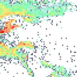
Elevation map (unit: m/reference plane: NAP, Western Scheldt, 2012) (Scheldemonitor:WSbi12TTGD20)
Elevation map of the Western Scheldt, containing both the sand banks, shoals and river depths. (unit: m/reference plane: NAP)
Luchtfoto Westkust (HistorischeKaarten:Westkust_mosaic)
Luchtfoto Zeebrugge, tijdens raid (HistorischeKaarten:ZB_Raid)
Luchtfoto Zeebrugge, geen raid (HistorischeKaarten:ZB_noRaid)
Zeekaart der Visscherij van Blankenberghe (HistorischeKaarten:Zeekaart_Vis_Bl)
Map made by E.H. Carlier, G. in the 19° century. More information through the metadata and on the website of HisGISKust.
Dataportal - Abiotic observations (Dataportal:abiotic_observations)
GOODS Abyssal Provinces (World:abyssalprovinces)
The abyssal provinces are separated by mid-ocean ridges and other bathyal topography creating deep basins and/or are distinguished by varying levels of POC flux to the seafloor. Source: Watling, L.; Guinotte, J.; Clark, M.R.; Smith, C.R. (2013). A proposed biogeography of the deep ocean floor. Prog. Oceanogr. 111: 91-112. hdl.handle.net/10.1016/j.pocean.2012.11.003 In: Progress in Oceanography. Pergamon: Oxford. ISSN 0079-6611
EMODnet Relative abundance Acartia spp. masked with relative error 0.3 (North Atlantic, 1958-2016) (Emodnetbio:aca_spp_19582016_L1)
Gridded abundance map of Acartia spp. This product was developed with DIVA (Data-Interpolating Variational Analysis). Data was provided by SAHFOS (Continuous Plankton Recorder) for use as an ICES operational oceanographic product.
EMODnet Relative abundance Acartia spp. masked with relative error 0.3 (North Atlantic, 1958-2016) (Emodnetbio:aca_spp_19582016_L1_err)
Gridded abundance map of Acartia spp. This product was developed with DIVA (Data-Interpolating Variational Analysis). Data was provided by SAHFOS (Continuous Plankton Recorder) for use as an ICES operational oceanographic product.
Antarctic Conservation Biogeographic Regions (ACBRs, Antarctica, 2017) (Antarctica:acbr_v2_2016)
Citation: Terauds, A. (2016, updated 2017) An update of the Antarctic Conservation Biogeographic Regions (ACBRs) Australian Antarctic Data Centre - doi:10.4225/15/5729930925224
Accommodation capacity 2000-2012 (Al Hoceima) (Morocco:accomodationcapacity)
Accommodation capacity 2000-2012 Al Hoceima
Administrative boundaries IZemouren, Al Hoceima, Youssed Ou Ali, Imzouren, Bni Bouyach, Trougout (Morocco:admin_boundary)
Administrative boundaries Al Hoceima, Trougout, Izemouren, Youssed Ou Ali, BNI Bouyach, Imzouren
Afstanden vanaf Vlissingen (VLIZ, 2009) (Scheldemonitor:afstanden_vlissingen)
Aéroport Charif Idrissi, Al Hoceima (Morocco:airoport)
Airport Al Hoceima CASE - PEGASOproject
Built-up in Al Hoceima (2012) (Morocco:al_hoceima_urbain)
Urban Al Hoceima; Al Hoceima CASE - PEGASOproject
Temporal Turnover in European Macrobenthos Communities (Emodnetbio:all_diversity_measures)
This product builds on the EMODnet Biology data product Presence/absence data of macrozoobenthos in the European Seas to derive estimates of temporal turnover in benthic communities on a spatial grid across European seas. This product only uses species-level records, and only uses sampling events where the full macrobenthic community was surveyed (i.e. where there are no 'NA' values in the presence/absence dataset for any species). Six time periods are considered, based on data availability: before 1990, 1990-1999, 2000-2004, 2005-2009, 2010-2014, and 2015 and after. A 1 degree grid is used to obtain reasonable numbers of repeat samples per grid cell. The code below could be adapted to set different time periods and/or a different grid resolution. This readme describes the product structure, including the workflow to generate the required derived datasets and the process for turning them into gridded maps of community turnover.
Share of single person households (Belgian coastal area, 2018-2022) (Kustportaal:alleenstaandehuish_34)
Proportion of single households. Source: FOD Binnenlandse zaken, Algemene Directie Instellingen en Bevolking, Rijksregister
TBD - Ankerplaatsen Noordzee (NorthSea:ankerplaats)
International Bathymetric Chart of the Southern Ocean (IBCSO) (IBCSO:antarctica_background)
Arndt, J.E., H. W. Schenke, M. Jakobsson, F. Nitsche, G. Buys, B. Goleby, M. Rebesco, F. Bohoyo, J.K. Hong, J. Black, R. Greku, G. Udintsev, F. Barrios, W. Reynoso-Peralta, T. Morishita, R. Wigley, "The International Bathymetric Chart of the Southern Ocean (IBCSO) Version 1.0 - A new bathymetric compilation covering circum-Antarctic waters", Geophysical Research Letters, doi: 10.1002/grl.50413
Antarctic territorial claims (Antarctica:antarctica_claims)
This GIS layer contains polygons with claimed areas by different nations. Based on information from: http://gcmd.nasa.gov/KeywordSearch/Metadata.do?Portal=amd&KeywordPath=Parameters%7CHUMAN+DIMENSIONS%7CENVIRONMENTAL+GOVERNANCE%2FMANAGEMENT&EntryId=%5BAADC%5Dgis108&MetadataView=Full&MetadataType=0&lbnode=mdlb1, adapted by VLIZ
Port of Antwerp (Antwerp, 2008) (Scheldemonitor:antwerpharbour)
Water area in front of the port of Antwerp based on the ESRI - Europe Water.
Share of appartments (Belgian coastal area, 2018-2022) (Kustportaal:appartementen_37)
The proportion of appartments against the different types of housing. Source: FOD Financiën, Administratie van het kadaster, de registratie en de domeinen
aquamaps (World:aquamaps)
Arctic Marine Areas (MarineRegions:arcticmarineareas)
There are many ways to divide the Arctic marine region—by ecosystem/ecological characteristics, by administrative criteria, or by some combination of the two. However, effective monitoring of biodiversity requires that an ecosystem-based approach be used for choosing areas. http://geo.abds.is/geonetwork/srv/eng/catalog.search#/metadata/dcd5c12f-3acb-4101-8e1a-bba0aec50582
AZMP (Atlantic Zone Monitoring Program) Sections (WoRMS:azmp_sections)
Fisheries and Oceans Canada. (2014). Atlantic Zone Monitoring Program Website. Retrieved 4 December 2014 from Fisheries and Oceans Canada.
Bathing areas (Belgian coast, 2013) (Kustportaal:badzones_buffer250m)
The displayed bathing areas are based on the Provincial Spatial Implementation Plan 'Strand en Dijk 2013'.
Dredging and dumping sites (Belgian part of North Sea, 2012) (Kustportaal:baggerlocaties_2012)
The location of dredging and dumping sites in the BNS for the year 2012.
Dredging and dumping sites (Belgian part of North Sea, 2013) (Kustportaal:baggerlocaties_2013)
The location of dredging and dumping sites in the BNS for the year 2013.
Dredging and dumping sites (Belgian part of North Sea, 2014) (Kustportaal:baggerlocaties_2014)
The location of dredging and dumping sites in the BNS for the year 2014.
Dredging and dumping sites (Belgian part of North Sea, 2015) (Kustportaal:baggerlocaties_2015)
The location of dredging and dumping sites in the BNS for the year 2015.
Dredging and dumping sites (Belgian part of North Sea, 2016) (Kustportaal:baggerlocaties_2016)
The location of dredging and dumping sites in the BNS for the year 2016.
Dredging Zone, Belgian Continental Shelf (NorthSea:baggerzonesbcp)
Banks of the Southern Bight of the North Sea (NorthSea:banks)
Sub-watershed Drainage Basins for Baltic Sea drainage basin region (Pesi:basinsbalticsea)
The main Baltic Sea drainage basin map was created by M. Falkenmark and Z. Mikulski (HELCOM 1986). Both map projection and scale are unknown. Independent measurements indicate a scale of approximately 1:5,000,000. Two additional maps were used to provide more accurate delineations in the Danish Straits and Kattegat sub- regions. These paper maps were also of unknown scale and projection. The Digital Chart of the World (DCW) by ESRI was used for spatial positioning when joining all data sets. These map sources identified 81 sub-basins, which can be aggregated to seven major watersheds for the following major water bodies that define the Baltic Sea: Bothnian Bay, Bothnian Sea, Gulf of Finland, Gulf of Riga, the Baltic Proper, Danish Straits, and the Kattegat. The main Baltic Sea drainage basin map was digitised and transformed in three separate sections using PC ARC/INFO. The Root Mean Square (RMS) error ranged between 0.01 and 0.02. Four sub- basins from the Danish Straits and nine from the Kattegat paper maps were digitised. The RMS errors were 0.01 and 0.06, respectively. All sections were joined together using the APPEND command. Although some RMS errors were high, the final drainage basin data set lines up well with other coverages in the database. The coverage was edited for dangling arcs and label errors. When the editing process was complete, topology was created using the CLEAN command with a 20 meter fuzzy tolerance and dangle length. All polygons were assigned unique id's before attribute data was added. An item called SUBID was added to the coverages .PAT file. This value represents the sub-basin or water body for which each polygon belongs. SUBID served as a bridge item to join additional attributes that existed in an EXCEL spreadsheet. Individual SUBIDs were assigned by selecting polygon label points in ARCEDIT and CALCing SUBID to be the correct value. Extensive error checking was performed before all other attribute data was appended. In addition to the added item SUBID, 21 other attributes were appended to the cover .PAT file. These attributes originated from (a) and database of monthly loads of land based eutrophying substances (Stalnache, 1994), (b) data extracted from the Land Cover data set, and (c) data extracted from the Population Distribution data set. The final BASINS coverage has a total of 26 attributes, including the four automatically generated by ARC/INFO. Supplier: GRID-Arendal. PO Box 1602, Myrene. N-4801 Arendal, Norway.
Quality of bathing water at Calabonita Beach and Quemado Beach (1993-2011) (Morocco:bathingquality)
Quality of bathing water (1993-2011)
MARSPEC: global marine bathymetry (MARSPEC:bathy_30s1)
Footprints bathymetric surveys VLIZ (Belgian part of North Sea, 2012-2022) (Kustportaal:bathy_vliz_bpns)
This layer contains the footprints of bathymetric surveys performed by VLIZ in the period 2012-2022 in the Belgian part of the North Sea. The bathymetric data gathered during these surveys is available for download in the Marine Data Archive (mda.vliz.be). For more information on the data acquisition, contact infrastructuur@vliz.be. For access to MDA, contact data@vliz.be.
Footprints bathymetric surveys wrecks VLIZ (Belgian part of North Sea, 2012-2018) (Kustportaal:bathy_vliz_wrecks)
This layer contains the footprints of bathymetric surveys of shipwrecks performed by VLIZ in the period 2012-2018 in the Belgian part of the North Sea. The bathymetric data gathered during these surveys is available for download in the Marine Data Archive (mda.vliz.be). For more information on the data acquisition, contact infrastructuur@vliz.be. For access to MDA, contact data@vliz.be.
Bathymetry (EMODnet, Belgian part of North Sea, 2018) (Kustportaal:bathymetry_belgianpartnorthsea)
This DTM was released by the EMODnet Bathymetry portal in September 2018 and has a grid resolution of 1/16 * 1/16 arc minutes (circa 115 * 115 meters).
Bathymetric difference map (unit: dm, Paardenmarkt, 1855-1825) (Paardenmarkt:bathymetry_diff_1855-1825)
The difference map between 1825 and 1855 is created based on depth measurements of the two historical bathymetry maps ‘Water depths Cotes-des-Pays-Bas, Reprductie Beautemps-Beaupré 1825’ and ‘L' Embouchure de L' Escaut, Marine Néerlandaise 1855’. This map is created to further look into the dynamics and evolution of the seabed. Red colours indicate erosion whereas green colours indicate sedimentation (in decimeters). For the interpolation process the same mask layer was used. to make sure that the resolutions of the new depth layers were similar. This was done in order to perform raster calculations with the new depth maps to further observe changes on the seabed between these maps. Thus, the difference map represents the height differences over time of the seabed between an older and a newer map. There are three time series: (1) period 1825 – 1996 in ~10-year steps; (2) period 1968-1980 in 1-4-year steps; (3) period 1904-1996 in ~50-year steps.
Bathymetric difference map (unit: dm, Paardenmarkt, 1865-1855) (Paardenmarkt:bathymetry_diff_1865-1855)
The difference map between 1855 and 1865 is created based on depth measurements of the two historical bathymetry maps ‘L' Embouchure de L' Escaut, Marine Néerlandaise 1855’ and ‘L' Embouchure de L' Escaut, Marine Néerlandaise 1865’. This map is created to further look into the dynamics and evolution of the seabed. Red colours indicate erosion whereas green colours indicate sedimentation (in decimeters). For the interpolation process the same mask layer was used. to make sure that the resolutions of the new depth layers were similar. This was done in order to perform raster calculations with the new depth maps to further observe changes on the seabed between these maps. Thus, the difference map represents the height differences over time of the seabed between an older and a newer map.
Bathymetric difference map (unit: dm, Paardenmarkt, 1878-1865) (Paardenmarkt:bathymetry_diff_1878-1865)
The difference map between 1865 and 1878 is created based on depth measurements of the two historical bathymetry maps ‘L' Embouchure de L' Escaut, Marine Néerlandaise 1865’ and ‘L' Embouchure de L' Escaut, Marine Néerlandaise 1878’. This map is created to further look into the dynamics and evolution of the seabed. Red colours indicate erosion whereas green colours indicate sedimentation (in decimeters). For the interpolation process the same mask layer was used. to make sure that the resolutions of the new depth layers were similar. This was done in order to perform raster calculations with the new depth maps to further observe changes on the seabed between these maps. Thus, the difference map represents the height differences over time of the seabed between an older and a newer map.
Bathymetric difference map (unit: dm, Paardenmarkt, 1895-1878) (Paardenmarkt:bathymetry_diff_1895-1878)
The difference map between 1878 and 1895 is created based on depth measurements of the two historical bathymetry maps ‘L' Embouchure de L' Escaut, Marine Néerlandaise 1878’ and ‘Zeegat van Vlissingen, J. M. Phaff, H. O. W. Planten en E. E. Dullemond 1895’. This map is created to further look into the dynamics and evolution of the seabed. Red colours indicate erosion whereas green colours indicate sedimentation (in decimeters). For the interpolation process the same mask layer was used. to make sure that the resolutions of the new depth layers were similar. This was done in order to perform raster calculations with the new depth maps to further observe changes on the seabed between these maps. Thus, the difference map represents the height differences over time of the seabed between an older and a newer map.
Bathymetric difference map (unit: dm, Paardenmarkt, 1904-1895) (Paardenmarkt:bathymetry_diff_1904-1895)
The difference map between 1895 and 1904 is created based on depth measurements of the two historical bathymetry maps ‘Zeegat van Vlissingen, J. M. Phaff, H. O. W. Planten en E. E. Dullemond 1895’ and ‘Rade de Heyst 1904’. This map is created to further look into the dynamics and evolution of the seabed. Red colours indicate erosion whereas green colours indicate sedimentation (in decimeters). For the interpolation process the same mask layer was used. to make sure that the resolutions of the new depth layers were similar. This was done in order to perform raster calculations with the new depth maps to further observe changes on the seabed between these maps. Thus, the difference map represents the height differences over time of the seabed between an older and a newer map.
Bathymetric difference map (unit: dm, Paardenmarkt, 1949-1904) (Paardenmarkt:bathymetry_diff_1949-1904)
The difference map between 1904 and 1949 is created based on depth measurements of the two historical bathymetry maps ‘Rade de Heyst 1904’ and ‘Gravelines - Westkapelle, Hydrografie Noordzee 1949’. This map is created to further look into the dynamics and evolution of the seabed. Red colours indicate erosion whereas green colours indicate sedimentation (in decimeters). For the interpolation process the same mask layer was used. to make sure that the resolutions of the new depth layers were similar. This was done in order to perform raster calculations with the new depth maps to further observe changes on the seabed between these maps. Thus, the difference map represents the height differences over time of the seabed between an older and a newer map.
Bathymetric difference map (unit: dm, Paardenmarkt, 1954-1904) (Paardenmarkt:bathymetry_diff_1954-1904)
The difference map between 1904 and 1954 is created based on depth measurements of the two historical bathymetry maps ‘Rade de Heyst 1904’ and ‘De Haan - Nederlandse grens, Hydrografische dienst der Kust Oostende’. This map is created to further look into the dynamics and evolution of the seabed. Red colours indicate erosion whereas green colours indicate sedimentation (in decimeters). For the interpolation process the same mask layer was used. to make sure that the resolutions of the new depth layers were similar. This was done in order to perform raster calculations with the new depth maps to further observe changes on the seabed between these maps. Thus, the difference map represents the height differences over time of the seabed between an older and a newer map.
Bathymetric difference map (unit: dm, Paardenmarkt, 1959-1949) (Paardenmarkt:bathymetry_diff_1959-1949)
The difference map between 1949 and 1959 is created based on depth measurements of the two historical bathymetry maps ‘Gravelines - Westkapelle, Hydrografie Noordzee 1949’ and ‘Vlaamse Banken - Hydrografische Dienst der Kust Oostende (metingen 1935-1965)’. This map is created to further look into the dynamics and evolution of the seabed. Red colours indicate erosion whereas green colours indicate sedimentation (in decimeters). For the interpolation process the same mask layer was used. to make sure that the resolutions of the new depth layers were similar. This was done in order to perform raster calculations with the new depth maps to further observe changes on the seabed between these maps. Thus, the difference map represents the height differences over time of the seabed between an older and a newer map.
Bathymetric difference map (unit: dm, Paardenmarkt, 1968-1959) (Paardenmarkt:bathymetry_diff_1968-1959)
The difference map between 1959 and 1968 is created based on depth measurements of the two historical bathymetry maps ‘Vlaamse Banken - Hydrografische Dienst der Kust Oostende (metingen 1935-1965)’ and ‘Vlaamse Banken - Hydrografische Dienst der Kust Oostende (metingen 1935-1967)’. This map is created to further look into the dynamics and evolution of the seabed. Red colours indicate erosion whereas green colours indicate sedimentation (in decimeters). For the interpolation process the same mask layer was used. to make sure that the resolutions of the new depth layers were similar. This was done in order to perform raster calculations with the new depth maps to further observe changes on the seabed between these maps. Thus, the difference map represents the height differences over time of the seabed between an older and a newer map.
Bathymetric difference map (unit: dm, Paardenmarkt, 1971-1968) (Paardenmarkt:bathymetry_diff_1971-1968)
The difference map between 1968 and 1971 is created based on depth measurements of the two historical bathymetry maps ‘Vlaamse Banken - Hydrografische Dienst der Kust Oostende (metingen 1935-1967)’ and ‘Vlaamse Banken - Hydrografische Dienst der Kust Oostende (metingen 1959-1971)’. This map is created to further look into the dynamics and evolution of the seabed. Red colours indicate erosion whereas green colours indicate sedimentation (in decimeters). For the interpolation process the same mask layer was used. to make sure that the resolutions of the new depth layers were similar. This was done in order to perform raster calculations with the new depth maps to further observe changes on the seabed between these maps. Thus, the difference map represents the height differences over time of the seabed between an older and a newer map.
Bathymetric difference map (unit: dm, Paardenmarkt, 1972-1904) (Paardenmarkt:bathymetry_diff_1972-1904)
The difference map between 1904 and 1972 is created based on depth measurements of the two historical bathymetry maps ‘Rade de Heyst 1904’ and ‘Belgische- Ne kust, Monding der Westerschelde, Dienst der Kust Oostende 1972’. This map is created to further look into the dynamics and evolution of the seabed. Red colours indicate erosion whereas green colours indicate sedimentation (in decimeters). For the interpolation process the same mask layer was used. to make sure that the resolutions of the new depth layers were similar. This was done in order to perform raster calculations with the new depth maps to further observe changes on the seabed between these maps. Thus, the difference map represents the height differences over time of the seabed between an older and a newer map.
Bathymetric difference map (unit: dm, Paardenmarkt, 1972-1971) (Paardenmarkt:bathymetry_diff_1972-1971)
The difference map between 1971 and 1972 is created based on depth measurements of the two historical bathymetry maps ‘Vlaamse Banken - Hydrografische Dienst der Kust Oostende (metingen 1959-1971)’ and ‘Belgische- Ne kust, Monding der Westerschelde, Dienst der Kust Oostende 1972’. This map is created to further look into the dynamics and evolution of the seabed. Red colours indicate erosion whereas green colours indicate sedimentation (in decimeters). For the interpolation process the same mask layer was used. to make sure that the resolutions of the new depth layers were similar. This was done in order to perform raster calculations with the new depth maps to further observe changes on the seabed between these maps. Thus, the difference map represents the height differences over time of the seabed between an older and a newer map.
Bathymetric difference map (unit: dm, Paardenmarkt, 1973-1972) (Paardenmarkt:bathymetry_diff_1973-1972)
The difference map between 1972 and 1973 is created based on depth measurements of the two historical bathymetry maps ‘Belgische- Ne kust, Monding der Westerschelde, Dienst der Kust Oostende 1972’ and ‘Vlaamse Banken - Hydrografische Dienst der Kust Oostende (metingen 1959-1972)’. This map is created to further look into the dynamics and evolution of the seabed. Red colours indicate erosion whereas green colours indicate sedimentation (in decimeters). For the interpolation process the same mask layer was used. to make sure that the resolutions of the new depth layers were similar. This was done in order to perform raster calculations with the new depth maps to further observe changes on the seabed between these maps. Thus, the difference map represents the height differences over time of the seabed between an older and a newer map.
Bathymetric difference map (unit: dm, Paardenmarkt, 1974-1973) (Paardenmarkt:bathymetry_diff_1974-1973)
The difference map between 1973 and 1974 is created based on depth measurements of the two historical bathymetry maps ‘Vlaamse Banken - Hydrografische Dienst der Kust Oostende (metingen 1959-1972)’ and ‘Vlaamse Banken - Hydrografische Dienst der Kust Oostende (metingen 1959-1973)’. This map is created to further look into the dynamics and evolution of the seabed. Red colours indicate erosion whereas green colours indicate sedimentation (in decimeters). For the interpolation process the same mask layer was used. to make sure that the resolutions of the new depth layers were similar. This was done in order to perform raster calculations with the new depth maps to further observe changes on the seabed between these maps. Thus, the difference map represents the height differences over time of the seabed between an older and a newer map.
Bathymetric difference map (unit: dm, Paardenmarkt, 1980-1974) (Paardenmarkt:bathymetry_diff_1980-1974)
The difference map between 1974 and 1980 is created based on depth measurements of the two historical bathymetry maps ‘Vlaamse Banken - Hydrografische Dienst der Kust Oostende (metingen 1959-1973)’ and ‘Vlaamse Banken - Hydrografische Dienst der Kust Oostende (metingen 1959-1979)’. This map is created to further look into the dynamics and evolution of the seabed. Red colours indicate erosion whereas green colours indicate sedimentation (in decimeters). For the interpolation process the same mask layer was used. to make sure that the resolutions of the new depth layers were similar. This was done in order to perform raster calculations with the new depth maps to further observe changes on the seabed between these maps. Thus, the difference map represents the height differences over time of the seabed between an older and a newer map.
Bathymetric difference map (unit: dm, Paardenmarkt, 1981-1968) (Paardenmarkt:bathymetry_diff_1981-1968)
The difference map between 1968 and 1981 is created based on depth measurements of the two historical bathymetry maps ‘Vlaamse Banken - Hydrografische Dienst der Kust Oostende (metingen 1935-1967)’ and ‘Belgische- Ne kust, Monding der Westerschelde Dienst der Kust Oostende (metingen 1967-1981)’. This map is created to further look into the dynamics and evolution of the seabed. Red colours indicate erosion whereas green colours indicate sedimentation (in decimeters). For the interpolation process the same mask layer was used. to make sure that the resolutions of the new depth layers were similar. This was done in order to perform raster calculations with the new depth maps to further observe changes on the seabed between these maps. Thus, the difference map represents the height differences over time of the seabed between an older and a newer map.
Bathymetric difference map (unit: dm, Paardenmarkt, 1996-1904) (Paardenmarkt:bathymetry_diff_1996-1904)
The difference map between 1904 and 1996 is created based on depth measurements of the two historical bathymetry maps ‘Rade de Heyst 1904’ and ‘Vlaamse Banken - Hydrografische Dienst der Kust Oostende 1996’. This map is created to further look into the dynamics and evolution of the seabed. Red colours indicate erosion whereas green colours indicate sedimentation (in decimeters). For the interpolation process the same mask layer was used. to make sure that the resolutions of the new depth layers were similar. This was done in order to perform raster calculations with the new depth maps to further observe changes on the seabed between these maps. Thus, the difference map represents the height differences over time of the seabed between an older and a newer map.
Bathymetric difference map (unit: dm, Paardenmarkt, 1996-1954) (Paardenmarkt:bathymetry_diff_1996-1954)
The difference map between 1954 and 1996 is created based on depth measurements of the two historical bathymetry maps ‘De Haan - Nederlandse grens, Hydrografische dienst der Kust Oostende 1954’ and ‘Vlaamse Banken - Hydrografische Dienst der Kust Oostende 1996’. This map is created to further look into the dynamics and evolution of the seabed. Red colours indicate erosion whereas green colours indicate sedimentation (in decimeters). For the interpolation process the same mask layer was used. to make sure that the resolutions of the new depth layers were similar. This was done in order to perform raster calculations with the new depth maps to further observe changes on the seabed between these maps. Thus, the difference map represents the height differences over time of the seabed between an older and a newer map.
Bathymetric difference map (unit: dm, Paardenmarkt, 1996-1972) (Paardenmarkt:bathymetry_diff_1996-1972)
The difference map between 1972 and 1996 is created based on depth measurements of the two historical bathymetry maps ‘Belgische- Ne kust, Monding der Westerschelde, Dienst der Kust Oostende 1972’ and ‘Vlaamse Banken - Hydrografische Dienst der Kust Oostende 1996’. This map is created to further look into the dynamics and evolution of the seabed. Red colours indicate erosion whereas green colours indicate sedimentation (in decimeters). For the interpolation process the same mask layer was used. to make sure that the resolutions of the new depth layers were similar. This was done in order to perform raster calculations with the new depth maps to further observe changes on the seabed between these maps. Thus, the difference map represents the height differences over time of the seabed between an older and a newer map.
Bathymetric difference map (unit: dm, Paardenmarkt, 1996VB-1981) (Paardenmarkt:bathymetry_diff_1996VB-1981)
The difference map between 1981 and 1996 is created based on depth measurements of the two historical bathymetry maps ‘Belgische- Ne kust, Monding der Westerschelde Dienst der Kust Oostende (metingen 1967-1981)’ and ‘Vlaamse Banken - Hydrografische Dienst der Kust Oostende 1996’. This map is created to further look into the dynamics and evolution of the seabed. Red colours indicate erosion whereas green colours indicate sedimentation (in decimeters). For the interpolation process the same mask layer was used. to make sure that the resolutions of the new depth layers were similar. This was done in order to perform raster calculations with the new depth maps to further observe changes on the seabed between these maps. Thus, the difference map represents the height differences over time of the seabed between an older and a newer map.
Bathymetry (unit: dm/reference plane: GLLWS, Paardenmarkt, 1811) (Paardenmarkt:bathymetry_gllws_1811)
Water depths of the Paardenmarkt area in the year 1811. Bathymetry map is based on the georeferenced historical maps ‘Water depths Cotes-des-Pays-Bas, Reprductie Beautemps-Beaupré’ containing depth measurements. The depth values on all the maps are measured from the chart datum mean lowest low water spring (GLLWS = ‘gemiddelde laag-laagwaterspring’). Interpolations of the vector points layers to raster layers was done with the GRASS function ‘v.surf.rst’ to create the bathymetrie map. The GRASS function interpolates a vector point maps, using splines, with a raster layer used as mask (https://grass.osgeo.org/grass78/manuals/v.surf.rst.html).
Bathymetry (unit: dm/reference plane: GLLWS, Paardenmarkt, 1825) (Paardenmarkt:bathymetry_gllws_1825)
Water depths of the Paardenmarkt area in the year 1825. Bathymetry map is based on the georeferenced historical maps ‘L' Embouchure de L' Escaut, Marine Néerlandaise’ containing depth measurements. The depth values on all the maps are measured from the chart datum mean lowest low water spring (GLLWS = ‘gemiddelde laag-laagwaterspring’). Interpolations of the vector points layers to raster layers was done with the GRASS function ‘v.surf.rst’ to create the bathymetrie map. The GRASS function interpolates a vector point maps, using splines, with a raster layer used as mask (https://grass.osgeo.org/grass78/manuals/v.surf.rst.html).
Bathymetry (unit: dm/reference plane: GLLWS, Paardenmarkt, 1842) (Paardenmarkt:bathymetry_gllws_1842)
Water depths of the Paardenmarkt area in the year 1842. Bathymetry map is based on the georeferenced historical ‘L' Embouchure de L' Escaut, Marine Néerlandaise’ containing depth measurements. The depth values on all the maps are measured from the chart datum mean lowest low water spring (GLLWS = ‘gemiddelde laag-laagwaterspring’). Interpolations of the vector points layers to raster layers was done with the GRASS function ‘v.surf.rst’ to create the bathymetrie map. The GRASS function interpolates a vector point maps, using splines, with a raster layer used as mask (https://grass.osgeo.org/grass78/manuals/v.surf.rst.html).
Bathymetry (unit: dm/reference plane: GLLWS, Paardenmarkt, 1855) (Paardenmarkt:bathymetry_gllws_1855)
Water depths of the Paardenmarkt area in the year 1855. Bathymetry map is based on the georeferenced historical maps ‘L' Embouchure de L' Escaut, Marine Néerlandaise’ containing depth measurements. The depth values on all the maps are measured from the chart datum mean lowest low water spring (GLLWS = ‘gemiddelde laag-laagwaterspring’). Interpolations of the vector points layers to raster layers was done with the GRASS function ‘v.surf.rst’ to create the bathymetrie map. The GRASS function interpolates a vector point maps, using splines, with a raster layer used as mask (https://grass.osgeo.org/grass78/manuals/v.surf.rst.html).
Bathymetry (unit: dm/reference plane: GLLWS, Paardenmarkt, 1865) (Paardenmarkt:bathymetry_gllws_1865)
Water depths of the Paardenmarkt area in the year 1865. Bathymetry map is based on the georeferenced historical maps ‘L' Embouchure de L' Escaut, Marine Néerlandaise’ containing depth measurements. The depth values on all the maps are measured from the chart datum mean lowest low water spring (GLLWS = ‘gemiddelde laag-laagwaterspring’). Interpolations of the vector points layers to raster layers was done with the GRASS function ‘v.surf.rst’ to create the bathymetrie map. The GRASS function interpolates a vector point maps, using splines, with a raster layer used as mask (https://grass.osgeo.org/grass78/manuals/v.surf.rst.html).
Bathymetry (unit: dm/reference plane: GLLWS, Paardenmarkt, 1878) (Paardenmarkt:bathymetry_gllws_1878)
Water depths of the Paardenmarkt area in the year 1878. Bathymetry map is based on the georeferenced historical maps ‘L' Embouchure de L' Escaut, Marine Néerlandaise’ containing depth measurements. The depth values on all the maps are measured from the chart datum mean lowest low water spring (GLLWS = ‘gemiddelde laag-laagwaterspring’). Interpolations of the vector points layers to raster layers was done with the GRASS function ‘v.surf.rst’ to create the bathymetrie map. The GRASS function interpolates a vector point maps, using splines, with a raster layer used as mask (https://grass.osgeo.org/grass78/manuals/v.surf.rst.html).
Bathymetry (unit: dm/reference plane: GLLWS, Paardenmarkt, 1895) (Paardenmarkt:bathymetry_gllws_1895)
Water depths of the Paardenmarkt area in the year 1895. Bathymetry map is based on the georeferenced historical maps ‘Zeegat van Vlissingen, J. M. Phaff, H. O. W. Planten en E. E. Dullemond’ containing depth measurements. The depth values on all the maps are measured from the chart datum mean lowest low water spring (GLLWS = ‘gemiddelde laag-laagwaterspring’). Interpolations of the vector points layers to raster layers was done with the GRASS function ‘v.surf.rst’ to create the bathymetrie map. The GRASS function interpolates a vector point maps, using splines, with a raster layer used as mask (https://grass.osgeo.org/grass78/manuals/v.surf.rst.html).
Bathymetry (unit: dm/reference plane: GLLWS, Paardenmarkt, 1904) (Paardenmarkt:bathymetry_gllws_1904)
Water depths of the Paardenmarkt area in the year 1904. Bathymetry map is based on the georeferenced historical maps ‘Rade de Heyst’ containing depth measurements. The depth values on all the maps are measured from the chart datum mean lowest low water spring (GLLWS = ‘gemiddelde laag-laagwaterspring’). Interpolations of the vector points layers to raster layers was done with the GRASS function ‘v.surf.rst’ to create the bathymetrie map. The GRASS function interpolates a vector point maps, using splines, with a raster layer used as mask (https://grass.osgeo.org/grass78/manuals/v.surf.rst.html).
Bathymetry (unit: dm/reference plane: GLLWS, Paardenmarkt, 1949) (Paardenmarkt:bathymetry_gllws_1949)
Water depths of the Paardenmarkt area in the year 1949. Bathymetry map is based on the georeferenced historical maps ‘Gravelines - Westkapelle, Hydrografie Noordzee’ containing depth measurements. The depth values on all the maps are measured from the chart datum mean lowest low water spring (GLLWS = ‘gemiddelde laag-laagwaterspring’). Interpolations of the vector points layers to raster layers was done with the GRASS function ‘v.surf.rst’ to create the bathymetrie map. The GRASS function interpolates a vector point maps, using splines, with a raster layer used as mask (https://grass.osgeo.org/grass78/manuals/v.surf.rst.html).
Bathymetry (unit: dm/reference plane: GLLWS, Paardenmarkt, 1954) (Paardenmarkt:bathymetry_gllws_1954)
Water depths of the Paardenmarkt area in the year 1954. Bathymetry map is based on the georeferenced historical maps ‘De Haan - Nederlandse grens, Hydrografische dienst der Kust Oostende’ containing depth measurements. The depth values on all the maps are measured from the chart datum mean lowest low water spring (GLLWS = ‘gemiddelde laag-laagwaterspring’). Interpolations of the vector points layers to raster layers was done with the GRASS function ‘v.surf.rst’ to create the bathymetrie map. The GRASS function interpolates a vector point maps, using splines, with a raster layer used as mask (https://grass.osgeo.org/grass78/manuals/v.surf.rst.html).
Bathymetry (unit: dm/reference plane: GLLWS, Paardenmarkt, 1959) (Paardenmarkt:bathymetry_gllws_1959)
Water depths of the Paardenmarkt area in the year 1959. Bathymetry map is based on the georeferenced historical maps ‘Vlaamse Banken - Hydrografische Dienst der Kust Oostende (metingen 1935-1965)’ containing depth measurements. The depth values on all the maps are measured from the chart datum mean lowest low water spring (GLLWS = ‘gemiddelde laag-laagwaterspring’). Interpolations of the vector points layers to raster layers was done with the GRASS function ‘v.surf.rst’ to create the bathymetrie map. The GRASS function interpolates a vector point maps, using splines, with a raster layer used as mask (https://grass.osgeo.org/grass78/manuals/v.surf.rst.html).
Bathymetry (unit: dm/reference plane: GLLWS, Paardenmarkt, 1960) (Paardenmarkt:bathymetry_gllws_1960)
Water depths of the Paardenmarkt area in the year 1960. Bathymetry map is based on the georeferenced historical maps ‘Mündung der Westerschelde, Deutschen Hydrographischen Inst’ containing depth measurements. The depth values on all the maps are measured from the chart datum mean lowest low water spring (GLLWS = ‘gemiddelde laag-laagwaterspring’). Interpolations of the vector points layers to raster layers was done with the GRASS function ‘v.surf.rst’ to create the bathymetrie map. The GRASS function interpolates a vector point maps, using splines, with a raster layer used as mask (https://grass.osgeo.org/grass78/manuals/v.surf.rst.html).
Bathymetry (unit: dm/reference plane: GLLWS, Paardenmarkt, 1966) (Paardenmarkt:bathymetry_gllws_1966)
Water depths of the Paardenmarkt area in the year 1966. Bathymetry map is based on the georeferenced historical maps ‘Vlaamse Banken - Hydrografische Dienst der Kust Oostende (metingen 1935-1965)’ containing depth measurements. The depth values on all the maps are measured from the chart datum mean lowest low water spring (GLLWS = ‘gemiddelde laag-laagwaterspring’). Interpolations of the vector points layers to raster layers was done with the GRASS function ‘v.surf.rst’ to create the bathymetrie map. The GRASS function interpolates a vector point maps, using splines, with a raster layer used as mask (https://grass.osgeo.org/grass78/manuals/v.surf.rst.html).
Bathymetry (unit: dm/reference plane: GLLWS, Paardenmarkt, 1968) (Paardenmarkt:bathymetry_gllws_1968)
Water depths of the Paardenmarkt area in the year 1968. Bathymetry map is based on the georeferenced historical maps ‘Vlaamse Banken - Hydrografische Dienst der Kust Oostende (metingen 1935-1967)’ containing depth measurements. The depth values on all the maps are measured from the chart datum mean lowest low water spring (GLLWS = ‘gemiddelde laag-laagwaterspring’). Interpolations of the vector points layers to raster layers was done with the GRASS function ‘v.surf.rst’ to create the bathymetrie map. The GRASS function interpolates a vector point maps, using splines, with a raster layer used as mask (https://grass.osgeo.org/grass78/manuals/v.surf.rst.html).
Bathymetry (unit: dm/reference plane: GLLWS, Paardenmarkt, 1971) (Paardenmarkt:bathymetry_gllws_1971)
Water depths of the Paardenmarkt area in the year 1971. Bathymetry map is based on the georeferenced historical maps ‘Vlaamse Banken - Hydrografische Dienst der Kust Oostende (metingen 1959-1971)’ containing depth measurements. The depth values on all the maps are measured from the chart datum mean lowest low water spring (GLLWS = ‘gemiddelde laag-laagwaterspring’). Interpolations of the vector points layers to raster layers was done with the GRASS function ‘v.surf.rst’ to create the bathymetrie map. The GRASS function interpolates a vector point maps, using splines, with a raster layer used as mask (https://grass.osgeo.org/grass78/manuals/v.surf.rst.html).
Bathymetry (unit: dm/reference plane: GLLWS, Paardenmarkt, 1972) (Paardenmarkt:bathymetry_gllws_1972)
Water depths of the Paardenmarkt area in the year 1972. Bathymetry map is based on the georeferenced historical maps ‘Belgische- Ne kust, Monding der Westerschelde, Dienst der Kust Oostende’ containing depth measurements. The depth values on all the maps are measured from the chart datum mean lowest low water spring (GLLWS = ‘gemiddelde laag-laagwaterspring’). Interpolations of the vector points layers to raster layers was done with the GRASS function ‘v.surf.rst’ to create the bathymetrie map. The GRASS function interpolates a vector point maps, using splines, with a raster layer used as mask (https://grass.osgeo.org/grass78/manuals/v.surf.rst.html).
Bathymetry (unit: dm/reference plane: GLLWS, Paardenmarkt, 1973) (Paardenmarkt:bathymetry_gllws_1973)
Water depths of the Paardenmarkt area in the year 1973. Bathymetry map is based on the georeferenced historical maps ‘Vlaamse Banken - Hydrografische Dienst der Kust Oostende (metingen 1959-1972)’ containing depth measurements. The depth values on all the maps are measured from the chart datum mean lowest low water spring (GLLWS = ‘gemiddelde laag-laagwaterspring’). Interpolations of the vector points layers to raster layers was done with the GRASS function ‘v.surf.rst’ to create the bathymetrie map. The GRASS function interpolates a vector point maps, using splines, with a raster layer used as mask (https://grass.osgeo.org/grass78/manuals/v.surf.rst.html).
Bathymetry (unit: dm/reference plane: GLLWS, Paardenmarkt, 1974) (Paardenmarkt:bathymetry_gllws_1974)
Water depths of the Paardenmarkt area in the year 1974. Bathymetry map is based on the georeferenced historical maps ‘Vlaamse Banken - Hydrografische Dienst der Kust Oostende (metingen 1959-1973)’ containing depth measurements. The depth values on all the maps are measured from the chart datum mean lowest low water spring (GLLWS = ‘gemiddelde laag-laagwaterspring’). Interpolations of the vector points layers to raster layers was done with the GRASS function ‘v.surf.rst’ to create the bathymetrie map. The GRASS function interpolates a vector point maps, using splines, with a raster layer used as mask (https://grass.osgeo.org/grass78/manuals/v.surf.rst.html).
Bathymetry (unit: dm/reference plane: GLLWS, Paardenmarkt, 1980) (Paardenmarkt:bathymetry_gllws_1980)
Water depths of the Paardenmarkt area in the year 1980. Bathymetry map is based on the georeferenced historical maps ‘Vlaamse Banken - Hydrografische Dienst der Kust Oostende (metingen 1959-1979)’ containing depth measurements. The depth values on all the maps are measured from the chart datum mean lowest low water spring (GLLWS = ‘gemiddelde laag-laagwaterspring’). Interpolations of the vector points layers to raster layers was done with the GRASS function ‘v.surf.rst’ to create the bathymetrie map. The GRASS function interpolates a vector point maps, using splines, with a raster layer used as mask (https://grass.osgeo.org/grass78/manuals/v.surf.rst.html).
Bathymetry (unit: dm/reference plane: GLLWS, Paardenmarkt, 1981) (Paardenmarkt:bathymetry_gllws_1981)
Water depths of the Paardenmarkt area in the year 1981. Bathymetry map is based on the georeferenced historical maps ‘Belgische- Ne kust, Monding der Westerschelde Dienst der Kust Oostende (metingen 1967-1981)’ containing depth measurements. The depth values on all the maps are measured from the chart datum mean lowest low water spring (GLLWS = ‘gemiddelde laag-laagwaterspring’). Interpolations of the vector points layers to raster layers was done with the GRASS function ‘v.surf.rst’ to create the bathymetrie map. The GRASS function interpolates a vector point maps, using splines, with a raster layer used as mask (https://grass.osgeo.org/grass78/manuals/v.surf.rst.html).
Bathymetry (unit: dm/reference plane: GLLWS, Paardenmarkt, 1982) (Paardenmarkt:bathymetry_gllws_1982)
Water depths of the Paardenmarkt area in the year 1982. Bathymetry map is based on the georeferenced historical maps ‘Vlaamse Banken - Hydrografische Dienst der Kust Oostende (metingen 1959-1981)’ containing depth measurements. The depth values on all the maps are measured from the chart datum mean lowest low water spring (GLLWS = ‘gemiddelde laag-laagwaterspring’). Interpolations of the vector points layers to raster layers was done with the GRASS function ‘v.surf.rst’ to create the bathymetrie map. The GRASS function interpolates a vector point maps, using splines, with a raster layer used as mask (https://grass.osgeo.org/grass78/manuals/v.surf.rst.html).
Bathymetry (unit: dm/reference plane: GLLWS, Paardenmarkt, 1984) (Paardenmarkt:bathymetry_gllws_1984)
Water depths of the Paardenmarkt area in the year 1984. Bathymetry map is based on the georeferenced historical maps ‘Vlaamse Banken - Hydrografische Dienst der Kust Oostende (metingen 1959-1983)’ containing depth measurements. The depth values on all the maps are measured from the chart datum mean lowest low water spring (GLLWS = ‘gemiddelde laag-laagwaterspring’). Interpolations of the vector points layers to raster layers was done with the GRASS function ‘v.surf.rst’ to create the bathymetrie map. The GRASS function interpolates a vector point maps, using splines, with a raster layer used as mask (https://grass.osgeo.org/grass78/manuals/v.surf.rst.html).
Bathymetry (unit: dm/reference plane: GLLWS, Paardenmarkt, 1985) (Paardenmarkt:bathymetry_gllws_1985)
Water depths of the Paardenmarkt area in the year 1985. Bathymetry map is based on the georeferenced historical maps ‘Monding van de Westerschelde - Hydrografische Dienst der Kust Oostende’ containing depth measurements. The depth values on all the maps are measured from the chart datum mean lowest low water spring (GLLWS = ‘gemiddelde laag-laagwaterspring’). Interpolations of the vector points layers to raster layers was done with the GRASS function ‘v.surf.rst’ to create the bathymetrie map. The GRASS function interpolates a vector point maps, using splines, with a raster layer used as mask (https://grass.osgeo.org/grass78/manuals/v.surf.rst.html).
Bathymetry (unit: dm/reference plane: GLLWS, Paardenmarkt, 1985) – Vlaamse Banken (Paardenmarkt:bathymetry_gllws_1985_VB)
Water depths of the Paardenmarkt area in the year 1985. Bathymetry map is based on the georeferenced historical maps ‘Vlaamse Banken - Hydrografische Dienst der Kust Oostende (metingen 1959-1983)’ containing depth measurements. The depth values on all the maps are measured from the chart datum mean lowest low water spring (GLLWS = ‘gemiddelde laag-laagwaterspring’). Interpolations of the vector points layers to raster layers was done with the GRASS function ‘v.surf.rst’ to create the bathymetrie map. The GRASS function interpolates a vector point maps, using splines, with a raster layer used as mask (https://grass.osgeo.org/grass78/manuals/v.surf.rst.html).
Bathymetry (unit: dm/reference plane: GLLWS, Paardenmarkt, 1988) (Paardenmarkt:bathymetry_gllws_1988)
Water depths of the Paardenmarkt area in the year 1988. Bathymetry map is based on the georeferenced historical maps ‘Vlaamse Banken - Hydrografische Dienst der Kust Oostende’ containing depth measurements. The depth values on all the maps are measured from the chart datum mean lowest low water spring (GLLWS = ‘gemiddelde laag-laagwaterspring’). Interpolations of the vector points layers to raster layers was done with the GRASS function ‘v.surf.rst’ to create the bathymetrie map. The GRASS function interpolates a vector point maps, using splines, with a raster layer used as mask (https://grass.osgeo.org/grass78/manuals/v.surf.rst.html).
Bathymetry (unit: dm/reference plane: GLLWS, Paardenmarkt, 1991) (Paardenmarkt:bathymetry_gllws_1991)
Water depths of the Paardenmarkt area in the year 1991. Bathymetry map is based on the georeferenced historical maps ‘Vlaamse Banken - Hydrografische Dienst der Kust Oostende’ containing depth measurements. The depth values on all the maps are measured from the chart datum mean lowest low water spring (GLLWS = ‘gemiddelde laag-laagwaterspring’). Interpolations of the vector points layers to raster layers was done with the GRASS function ‘v.surf.rst’ to create the bathymetrie map. The GRASS function interpolates a vector point maps, using splines, with a raster layer used as mask (https://grass.osgeo.org/grass78/manuals/v.surf.rst.html).
Bathymetry (unit: dm/reference plane: GLLWS, Paardenmarkt, 1996) (Paardenmarkt:bathymetry_gllws_1996)
Water depths of the Paardenmarkt area in the year 1996. Bathymetry map is based on the georeferenced historical maps ‘Vlaamse Banken - Hydrografische Dienst der Kust Oostende’ containing depth measurements. The depth values on all the maps are measured from the chart datum mean lowest low water spring (GLLWS = ‘gemiddelde laag-laagwaterspring’). Interpolations of the vector points layers to raster layers was done with the GRASS function ‘v.surf.rst’ to create the bathymetrie map. The GRASS function interpolates a vector point maps, using splines, with a raster layer used as mask (https://grass.osgeo.org/grass78/manuals/v.surf.rst.html).
Bathymetry (unit: m/reference plane: MLLWS, Southern Bight North Sea, 2000) (NorthSea:bathymetry_in)
Bathymetry of the Southern Bight of the North Sea, source: 'Limited Atlas of the Belgian Part of the North Sea, Maes et al., 2000, RUG - Instituut voor Natuurbehoud.'
Bathymetry (unit: m/reference plane: LAT, Paardenmarkt, 2013) (Paardenmarkt:bathymetry_lat_2013)
Water depth of the dumpsite area (2013). Multibeam survey performed by Magelas.
Bathymetry (unit: m/reference plane: LAT, Paardenmarkt, 2022) (Paardenmarkt:bathymetry_lat_2022)
Water depth of the dumpsite area (2022). Multibeam survey performed by GEOxyz.
Bathymetry (unit: m/reference plane: LAT, Paardenmarkt, 2023) (Paardenmarkt:bathymetry_lat_2023)
Water depth of the central dumpsite area (500x1000m area) (2023). Multibeam survey performed by GEOxyz.
High resolution North Sea bathymetry (lines) (NorthSea:bathymline)
North Sea bathymetry (polygons) (NorthSea:bathympoly)
Annual mean black carbon (BC) concentrations (Belgian coastal area, 2018) (Kustportaal:bc_anmean_2018_coastalzone)
Annual average of atmospheric black carbon concentration in um/m³ (source reference required). Source: VMM
Belgian Continental Shelf (NorthSea:bcs)
12 nautical mile limit (Belgian part of North Sea, 2015) (Belgium:be_12nm_2015)
Parallel line to the baseline at 12 nautical miles seaward. Source: Vlaamse Hydrografie
24 nautical mile limit (Belgian part of North Sea, 2015) (Belgium:be_24nm_2015)
Parallel line to the baseline at 24 nautical miles seaward. Source: Vlaamse Hydrografie
3 nautical mile limit (Belgian part of North Sea, 2015) (Belgium:be_3nm_2015)
Parallel line to the baseline at 3 nautical miles seaward. Source: Vlaamse Hydrografie
Baseline (Belgium, 2015) (Belgium:be_basislijn_2015)
The low-water mark (0 m depth line) and ends of permanent harbour works extending beyond the low-water mark. Source: Flemish Hydrography
Belgian part of the North Sea (Belgium, 2015) (Belgium:be_intgrens_2015)
Boundary of the Belgian territorial sea and the Belgian continental shelf with the Netherlands, United Kingdom and France. Source: Flemish Hydrography
Beach width along the Gulf of Al Hoceima (in meters) (Morocco:beach_width)
Beach width; Al Hoceima CASE - PEGASOproject
Share of built-up surface area (Belgian coastal area, 2000-2018) (Kustportaal:bebouwdopp_18)
Share of built-up surface area in the coastal and hinterland municipalities for each year. Source: FPS Economy, General Directorate of Statistics and Economic Information, based on the land register
Arrondissements (Belgium, 2014) (Belgium:belgium_arrondissements)
This dataset contains all the boundaries of all the Belgian arrondissements. It also contains the INS code and the French and Dutch name of each arrondissement. Source: ESRI Belux
Municipalities (Belgium, 2019) (Belgium:belgium_municipalities)
This dataset contains all the boundaries of all the Belgian municipalities. It also contains the INS code and the French and Dutch name of each municipality. Source: NGI, adapted after fusion Flemish municipalities (2019-01-01)
Provinces (Belgium, 2014) (Belgium:belgium_provinces)
This dataset contains all the boundaries of all the Belgian provinces. It also contains the INS code and the French and Dutch name of each province. Source: ESRI Belux
Coordinates of wind turbines currently built in windmill concession area Belwind Phase 1 (NorthSea:belwind_turbines_as_built)
Summary presence/absence maps of macro-endobenthos in European Seas, based on the EMODNET Biology database (Emodnetbio:benthos_europe)
The large databases of EMODNET Biology only store confirmed presences of taxon. However, when mapping taxon distribution, it is also important where the taxon did not occur: there is at least as much information in absences as in presences. Inferring absences from presence-only databases is difficult and always involves some guesswork. In this product we have used as much meta-information as possible to guide us in inferring absences. There is important meta-information at two different levels: the level of the data set, and the level of the taxon. Datasets can contain implicit information on absences when they have uniformly searched for the same taxon over a number of sample locations. Normally, if the taxon would have been present there, it would have been recorded. Other datasets, however, are not informative at all about absences. Typical examples are museum collections. The fact that a specimen is found at a particular place confirms that it lived there, but does not give information on any other taxon being present or absent in the same spot. A difficulty is that some datasets have searched for a restricted part of the total community, e.g. only sampled shellfish but no worms. In this case, absence of a shellfish taxon is relevant, but absence of a worm is not. The dataset can only be used to infer absence for the taxa it has targeted. Here we implicitly assume that a dataset inventorying the endomacrobenthos, is targeting all taxa belonging to this functional group. Usually, the distinction can be made on the basis of the metadata. It is also helpful to plot the total number of taxa versus the total number of samples. Incomplete datasets have far less taxa than expected for their size, compared to 'complete' datasets. At the taxon level, taxonomic registers such as WoRMS (WoRMS Editorial Board, 2021) give information on the functional group the taxon belongs to. This information is present for many taxa, but it is most likely incomplete. The size of the register excludes any easy test of completeness of the traits. However, even if incomplete, the register trait data can be used to select the most useful datasets. If one were to use an incomplete register directly to restrict the taxa to be used in mapping, that would cause loss of interesting information. Therefore the present workflow contains additional steps using the identified promising datasets rather than the taxon list based on the register’s traits.
Utilisation rate (Belgian coastal area, 2016) (Kustportaal:benuttingsgraad_38)
Share (%) of non-residential properties. Source: FOD Financiën, Administratie van het kadaster, de registratie en de domeinen
Population density (Scheldt municipalities, 2008) (Scheldemonitor:bevolking2008)
Population density of the Scheldt municipalities in 2008 as calculated in the project 'Indicators of the Long-Term Vision 2030 (LTV) of the Scheldt Estuary'.
Population density (Belgian coastal area, 2018-2022) (Kustportaal:bevolkingsdichth_33)
Number of inhabitants/km² Source: FOD Binnenlandse zaken, Algemene Directie Instellingen en Bevolking, Rijksregister
Evolution of population (Belgian coastal area, 2000-2022) (Kustportaal:bevolkingsevolutie_14)
Evolution of the population in the coastal area (coastal municipalities + hinterland municipalities). Source: rijksregister, processed by the province of West Flanders
bevolkingskern_2011 (Scheldemonitor:bevolkingskern_2011)
Population centers in the Netherlands in 2001 (Scheldemonitor:bevolkingskernen2001)
Bathymetry (unit: m/reference plane: LAT, Lower Sea Scheldt, 2017) (Scheldemonitor:bez_bth_lat_mt_2017_1m)
Bathymetric grid of the Beneden-Zeeschelde (Belgian border - Rupelmonde). Depths have positive values, heights negative. The resolution of the grid is 1 meter. The reference plane is LAT.
Bathymetry (unit: m/reference plane: LAT, Lower Sea Scheldt, 2018) (Scheldemonitor:bez_bth_lat_mt_2018_1m1)
Bathymetric grid of the Beneden-Zeeschelde (Belgian border - Rupelmonde). Depths have positive values, heights negative. The resolution of the grid is 1 meter. The reference plane is LAT.
Bathymetry (unit: m/reference plane: LAT, Lower Sea Scheldt, 2019) (Scheldemonitor:bez_bth_lat_mt_2019_1m1)
Bathymetric grid of the Beneden-Zeeschelde (Belgian border - Rupelmonde). Depths have positive values, heights negative. The resolution of the grid is 1 meter. The reference plane is LAT.
Dataportal - Biotic observations (Dataportal:biotic_observations)
Selection of European countries (Belgium, France, Netherlands, Luxembourg) (Scheldemonitor:bnful)
Boeien Vloot (2013) (NorthSea:boeien_vloot)
Buoys RWS (Western Scheldt, 2015) (Scheldemonitor:boeien_ws_rws_20150123)
Bathymetry (unit: m/reference plane: TAW, Upper Sea Scheldt, 2017) (Scheldemonitor:boz_bth_taw_mt_2017_1m)
Bathymetric grid of the Upper Sea Scheldt, between Rupelmonde and Ghent. Depths have positive values, heights negative. The resolution of the grid is 1 meter. The reference plane is TAW.
Bras d'Or Lake Biosphere Reserve [foutief] (MarineRegions:brasdorlakebiospherereserve)
What is the Bras d’Or Lake Biosphere Reserve? It is a UNESCO designated area defined by the watershed of the Bras d'Or lake. It is Canada's 16th biosphere. Biosphere reserves are special places around the world where people are trying to live more sustainably – that means 4 things: a healthy environment a healthy economy a healthy society a healthy culture The Bras d'Or Lake Biosphere Reserve Association is a group of volunteers who have worked to have the Bras d’Or Lake and its watershed designated as a UNESCO Man and the Biosphere Reserve. We now oversee the activities of the Biosphere Reserve. We are a registered society in the province of Nova Scotia. 532 Chebucto St. P.O. Box 711 Baddeck, NS B0E 1B0 Email: contact@blbra.ca Tel: (902) 674-2578 Canadian Biosphere Reserves Association The CBRA aims to help create healthy, sustainable communities across Canada while conserving our natural and cultural heritage by supporting Canadian biosphere reserves. In addition, the CBRA serves as a national and international voice for Canadian biosphere reserves. 422 Chemin des Moulins Mont-Saint-Hilaire, Quebec, J3G 4S6 Canada Website: www.biospherecanada.ca
Brazil States & Regions (World:brazil_states)
Broedparen per telgebied Westerschelde (Scheldemonitor:broedvogels_rikz_vdws7908)
Count of birds, Western Scheldt (2012/2013 -2019/2020) (Scheldemonitor:broedvogels_ws)
Counting areas of the counted or estimated numbers of non breeding birds in the Western Scheldt from 2012/2013 till 2019/2020.
Total gross tonnage of seagoing vessels per seaport (Belgium, 1980-2020) (Kustportaal:brutotonnage_06)
Total gross tonnage of the seagoing vessels per Flemish sea port. Source: Merckx, J.P. (2020). Zeehavens en luchthavens in Vlaanderen. Feiten, statistieken en indicatoren voor 2019. Mobiliteitsraad van Vlaanderen: Brussel. 195 pp.
Buffer (500 m) boeien MT (2010) (NorthSea:buffer_boeien_mt)
Buffer (500 m) boeien Vloot (2013) (NorthSea:buffer_boeien_vloot)
Neighbourhoods in the Netherlands (Scheldemonitor:buurten2008)
The marine biological valuation map of the Belgian Part of the North Sea (BWZee:bwzeeval)
Integrated marine biological valuation map for the Belgian part of the North Sea for seabirds, macrobenthos, epibenthos and demersal fish. BWZEE: A Biological Valuation Map for the Belgian Continental Shelf
EMODnet Relative abundance Calanus finmarchicus masked with relative error 0.3 (North Atlantic, 1958-2016) (Emodnetbio:cal_fin_19582016_L1_err)
Gridded abundance map of Calanus finmarchicus. This product was developed with DIVA (Data-Interpolating Variational Analysis). Data was provided by SAHFOS (Continuous Plankton Recorder) for use as an ICES operational oceanographic product.
EMODnet Relative abundance Calanus helgolandicus masked with relative error 0.3 (North Atlantic, 1958-2016) (Emodnetbio:cal_hel_19582016_L1_err)
Gridded abundance map of Calanus helgolandicus. This product was developed with DIVA (Data-Interpolating Variational Analysis). Data was provided by SAHFOS (Continuous Plankton Recorder) for use as an ICES operational oceanographic product.
Spatial interpolation of Calanus finmarchicus and Calanus helgolandicus observations in the North Sea (Emodnetbio:calanus_year_abundance)
Calcite (mean) [mol/m^3] (Bio-Oracle:calcite)
Calcite concentration indicates the mean concentration of calcite (CaCO3) in oceans. Derivation of metric: Mean Period: 2002-2009 Units: mol/m^3 Primary type: Satellite (Aqua-MODIS), seasonal climatologies Spatial resolution: 5 arcmin (9.2 km) Reference: (Feldman & McClain 2010) URL: http://oceancolor.gsfc.nasa.gov
Camping grounds (Flanders, 2018) (Kustportaal:campings_20180813)
Campsites with promotional attributes that may be relevant to the tourist. The licensed mini campsites according to the old Accommodation Decree have also been added to these datasets.
Camping grounds (Flanders, 2019) (Kustportaal:campings_20191209)
Campsites with promotional attributes that may be relevant to the tourist. The licensed mini campsites according to the old Accommodation Decree have also been added to these datasets.
Canadian provinces (World:canada_poly)
Global contourite distribution (World:cds)
Contourites are sedimentary units which are deposited or substantially reworked by alongslope bottom currents. They refer to the lithological unit and the terminology reflects the grain size of the sediment. Drifts refer to the same sedimentary unit as a contourite, but the word 'drift' reflects the morphological appearance of the sedimentary unit. Their terminology reflects the external shape, and the internal shape, which is determined by seismography. If drifts are clustered into a local area of certain size, we call the clustered sediment group a Contourite Depositional System (CDS). These sedimentary units are generally, but not exclusively, found in the deep sea (>2000m depth). They are a useful tool for determining paleoceanic and paleoclimatic changes, since their distribution is linked to bottom currents. They have gained interest from the hydrocarbon industry, since accumulation of source rocks may be influenced by bottom currents. Slope instability is also an area of interest for further research. Source methodology: For acquisition of the resulting information, several hundreds of papers on the relevant subject were read. Firstly, abstracts, introductions and conclusions were read for a general view on the article. Then further reading on the relevant chapters provided the presented information. In 2013, 166 records with the place type Drift were added to the Marine Gazetteer. These are linked to one of the 24 Contourite Depositional Systems, if they make part of such a system. Each drift is also influenced by a water mass or current. This water mass or current determines the sedimentation, erosion and movements of these sediments. In 2014, the list was extended with 81 records of the place type Drift. No Contourite Depositional Systems were added. The search process was identical to 2013, only this time a summary paper was the starting point (Rebesco et al., 2014). In this publication, the major drifts were listed with their most relevant sources along with them. These listed sources were then sought after and read. Not all papers were accessible at the time of this process, and thus it is advised to read these publications in the future as well.
Installation de Stockage des Déchets Non Dangereux (France) (Lifewatch:centrestockage_sinoe)
Source: Sinoe
Chemical sampling points (Paardenmarkt, 2003) (Paardenmarkt:chemsamplingpoints_2003)
Chemical sampling points (Paardenmarkt, 2005) (Paardenmarkt:chemsamplingpoints_2005)
Chemical sampling points (Paardenmarkt, 2007) (Paardenmarkt:chemsamplingpoints_2007)
Chemical sampling points (Paardenmarkt, 2008) (Paardenmarkt:chemsamplingpoints_2008)
Chemical sampling points (Paardenmarkt, 2009) (Paardenmarkt:chemsamplingpoints_2009)
Chemical sampling points (Paardenmarkt, 2010) (Paardenmarkt:chemsamplingpoints_2010)
Chemical sampling points (Paardenmarkt, 2011) (Paardenmarkt:chemsamplingpoints_2011)
Chemical sampling points (Paardenmarkt, 2013) (Paardenmarkt:chemsamplingpoints_2013)
Chemical sampling points (Paardenmarkt, 2014) (Paardenmarkt:chemsamplingpoints_2014)
Chemical sampling points (Paardenmarkt, 2015) (Paardenmarkt:chemsamplingpoints_2015)
Chemical sampling points (Paardenmarkt, 2016) (Paardenmarkt:chemsamplingpoints_2016)
Chemical sampling points (Paardenmarkt, 2017) (Paardenmarkt:chemsamplingpoints_2017)
Chemical sampling points (Paardenmarkt, 2018) (Paardenmarkt:chemsamplingpoints_2018)
Chemical sampling points (Paardenmarkt, 2019) (Paardenmarkt:chemsamplingpoints_2019)
Surface sediment sampling and bottom water sampling (2019). In total 19 points were sampled. Sampling performed by DOVO.
Chemical sampling points (Paardenmarkt, 2021) (Paardenmarkt:chemsamplingpoints_2021)
Surface sediment sampling and bottom water sampling (2021). In total 30 points were sampled. Sampling performed by DOVO.
Chemical sampling points (Paardenmarkt, 2022) (Paardenmarkt:chemsamplingpoints_2022)
Surface sediment sampling and bottom water sampling (2022). In total 30 points were sampled. Sampling performed by DOVO.
Chemical sampling points (Paardenmarkt, 2023) (Paardenmarkt:chemsamplingpoints_2023)
EMODnet Relative abundance chlorophyll index masked with relative error 0.3 (North Atlantic, 1958-2016) (Emodnetbio:chli_19582016_L1_err)
Gridded map of the abundance of the chlorophyll index. This product was developed with DIVA (Data-Interpolating Variational Analysis). Data was provided by SAHFOS (Continuous Plankton Recorder) for use as an ICES operational oceanographic product.
Chlorophyll A (maximum) [mol/m^3] (Bio-Oracle:chlomax)
Chlorophyll A concentration indicates the concentration of photosynthetic pigment chlorophyll A (the most common "green" chlorophyll) in oceans. Please note that in shallow water these values may reflect any kind of autotrophic biomass. Derivation of metric: Maximum Period: 2002-2009 Units: mol/m^3 Primary type: Satellite (Aqua-MODIS), monthly climatologies Spatial resolution: 5 arcmin (9.2 km) Reference: (Feldman & McClain 2010) URL: http://oceancolor.gsfc.nasa.gov/
Chlorophyll A (mean) [mol/m^3] (Bio-Oracle:chlomean)
Chlorophyll A concentration indicates the concentration of photosynthetic pigment chlorophyll A (the most common "green" chlorophyll) in oceans. Please note that in shallow water these values may reflect any kind of autotrophic biomass. Derivation of metric: Mean Period: 2002-2009 Units: mol/m^3 Primary type: Satellite (Aqua-MODIS), monthly climatologies Spatial resolution: 5 arcmin (9.2 km) Reference: (Feldman & McClain 2010) URL: http://oceancolor.gsfc.nasa.gov/
Chlorophyll A (minimum) [mol/m^3] (Bio-Oracle:chlomin)
Chlorophyll A concentration indicates the concentration of photosynthetic pigment chlorophyll A (the most common "green" chlorophyll) in oceans. Please note that in shallow water these values may reflect any kind of autotrophic biomass. Derivation of metric: Minimum Period: 2002-2009 Units: mol/m^3 Primary type: Satellite (Aqua-MODIS), monthly climatologies Spatial resolution: 5 arcmin (9.2 km) Reference: (Feldman & McClain 2010) URL: http://oceancolor.gsfc.nasa.gov/
Chlorophyll A (range) [mol/m^3] (Bio-Oracle:chlorange)
Chlorophyll A concentration indicates the concentration of photosynthetic pigment chlorophyll A (the most common "green" chlorophyll) in oceans. Please note that in shallow water these values may reflect any kind of autotrophic biomass. Derivation of metric: Range Period: 2002-2009 Units: mol/m^3 Primary type: Satellite (Aqua-MODIS), monthly climatologies Spatial resolution: 5 arcmin (9.2 km) Reference: (Feldman & McClain 2010) URL: http://oceancolor.gsfc.nasa.gov/
Seasonal chlorophyll values for 1980-2008 on a 1x1 degree grid (Emodnet:chlorophyll)
Extrapolated chlorophyll values for all seasons from 1980 to 2008 on a 1x1 degree grid for Europe, based on distinct surface chlorophyll data from Waterbase -Transitional, coastal and marine waters (European Environmental Agency). Waterbase is the generic name given to the EEA databases on the status and quality of Europe's rivers, lakes, groundwater bodies and transitional, coastal and marine waters, and on the quantity of Europe's water resources.
Seasonal chlorophyll point values for 1980-2008 (Emodnet:chlorophyllpoints)
Chlorophyll data points for all seasons from 1980 to 2008, based on chlorophyll data from Waterbase - Transitional, coastal and marine waters (European Environmental Agency). Waterbase is the generic name given to the EEA databases on the status and quality of Europe's rivers, lakes, groundwater bodies and transitional, coastal and marine waters, and on the quantity of Europe's water resources.
Cliffs on the Al Hoceima Area (Morocco:cliffs)
Cliffs Al Hoceima CASE - PEGASOproject
Cloud fraction (maximum) [%] (Bio-Oracle:cloudmax)
Cloud fraction indicates how much of the earth is covered by clouds. A bilinear interpolation was used to convert the data from 6 arcminutes to 5 arcminutes. Derivation of metric: Maximum Period: 2005-2010 Units: % Primary type: Satellite (Terra-MODIS), monthly images Spatial resolution: 6 arcmin Reference: (NASA 2010) URL: http://neo.sci.gsfc.nasa.gov/Search.html
Cloud fraction (mean) [%] (Bio-Oracle:cloudmean)
Cloud fraction indicates how much of the earth is covered by clouds. Derivation of metric: Mean Period: 2005-2011 Units: % Primary type: Satellite (Terra-MODIS), monthly images Spatial resolution: 6 arcmin Reference: (NASA 2010) URL: http://neo.sci.gsfc.nasa.gov/Search.html
Cloud fraction (minimum) [%] (Bio-Oracle:cloudmin)
Cloud fraction indicates how much of the earth is covered by clouds. Derivation of metric: Minimum Period: 2005-2012 Units: % Primary type: Satellite (Terra-MODIS), monthly images Spatial resolution: 6 arcmin Reference: (NASA 2010) URL: http://neo.sci.gsfc.nasa.gov/Search.html
Coastbusters mariculture project (Belgian part of North Sea, 2016-2019) (Kustportaal:coastbusters)
The Coastbusters pilot project (2016-2019) explores the use of innovative biostabilisation methods as a coastal protection mechanism, with the aim of achieving the natural increase of sand and strengthening the foreshores against coastal erosion.
TBD_Coastline 2006 (NorthSea:coastline_2006)
Coasts per ocean (20150814) (MarineRegions:coasts_per_ocean)
Coasts Subnational Level (20150814) (MarineRegions:coasts_subnational)
Continental margins between 140m and 3500m depth (MarineRegions:comarge)
This shapefile has been prepared in the framework of COMARGE, one of the field project of the Census of Marine Life. It is intended to represent continental margins worldwide, with the exclusion of the continental shelf. The continental margins have been defined based on bathymetry and expert opinion. The upper margin of the boundary has been set at 140 m depth, which is the average depth of the shelf break, except in Antarctica where the shelf break goes deeper and the upper boundary has been set up at 500 m. The lower boundary has been set at 3500 m depth. Both isobaths were extracted from S2004 Bathymetry (a global bathymetry at 1 arc-minute resolution). The upper and lower boundaries were manually edited to follow the contour of continental margins in particular cases. Please note that some but not all margins around island are included in this shapefile.
Concessie Thorntonbank (NorthSea:concessie_thornton)
Concession Zones Belgian Continental Shelf (NorthSea:concessiezones)
Concessiezones BCP (Feb2014) (NorthSea:concessiezones_201402)
Contour lines (zone 01, nature reserve Westhoek, 1983-1996) (Crestproject:contour_miwe01)
The contour lines of the map series 'Topography beach Flemish coast' were digitized by the Flanders Marine Institute, within the framework of the CREST-project . The maps were prepared by Eurosense Belfotop NV for Coastal Division and reflect the height model of the coastal zone of the Flemish coast, following coastal morphology for coastal defense and management of the coastal zone. For the height values, the reference plane Z was used. Note: only part of the file from 1996 was digitized.
Contour lines (zone 08, West-Groenendijk, 1983-1996) (Crestproject:contour_miwe08)
The contour lines of the map series 'Topography beach Flemish coast' were digitized by the Flanders Marine Institute, within the framework of the CREST-project . The maps were prepared by Eurosense Belfotop NV for Coastal Division and reflect the height model of the coastal zone of the Flemish coast, following coastal morphology for coastal defense and management of the coastal zone. For the height values, the reference plane Z was used.
Contour lines (zone 17-18, Mariakerke, 1983-1996) (Crestproject:contour_miwe1718)
The contour lines of the map series 'Topography beach Flemish coast' were digitized by the Flanders Marine Institute, within the framework of the CREST-project . The maps were prepared by Eurosense Belfotop NV for Coastal Division and reflect the height model of the coastal zone of the Flemish coast, following coastal morphology for coastal defense and management of the coastal zone. For the height values, the reference plane Z was used.
Coral reefs (MarineHeritage:coralreefs)
Sediment core sites (vibrocore, Paardenmarkt, 2020) (Paardenmarkt:corelocations_2020)
Shallow vibrocores from 8 sites surrounding the dumpsite (2020). Core acquisition by VLIZ.
SAHFOS CPR standard areas (Emodnet:cprgrid)
CPR standard areas are pre-defined areas used historically within the Continuous Plankton Recorder Survey. They include standar areas form the Gretar North Sea and North Atlnaic Ocean
Monitoring locations (CREST, Belgian coast, 2015-2019) (Crestproject:crest_monitoring)
This map shows the locations where measurements will be performed within the CREST project (Climate Resilient Coast). Different types of measurements will be carried out. * In Zeebrugge wave overtopping will be monitored. * Climatic parameters are collected in Ostend. * At Groenendijk-West and Mariakerke the amount of sand that is displaced under the influence of the wind will be measured. * In addition to these aeolian measurements, several parameters are measured in Mariakerke by means of buoys, and there is an Argus system operational. Every 30 minutes a photo is taken from the beach that can be used in the determination of the coastline, bathymetry and wave and current characteristics.
Test locations (CREST, Belgian coast, 2015-2019) (Crestproject:crest_testlocaties)
Two zones were defined in the CREST project (Climate Resilient Coast) as test sites. One zone is situated at Mariakerke, the other in West-Groenendijk (Koksijde). Following measurements will be carried out at both locations: measurements using wave buoys, with a frame, aeolian sand transport and wind and current measurements, topographic measurements.
Cross dateline features (polygons) (MarineRegions:cross_dateline_polygons)
Percentage of agricultural area relative to total area (Belgian coastal area, 1985-2021) (Kustportaal:cultuurgrond_22)
Percentage of the agricultural area relative to total area of the coastal and hinterland municipalities. Source: Department Agriculture and Fisheries based on FPS Economy, S.M.E.s, Self-employed and Energy – Statbel
A.K Khattabi Dam (Morocco:dam)
Dam; Al Hoceima CASE - PEGASOproject
Diffuse attenuation coefficient at 490 nm (maximum) [m^-1] (Bio-Oracle:damax)
The diffuse attenuation coefficient is an indicator of water clarity. It expresses how deeply visible light in the blue to the green region of the spectrum penetrates in to the water column. Derivation of metric: Maximum Period: 2002-2009 Units: m^-1 Primary type: Satellite (Aqua-MODIS), monthly climatologies Spatial resolution: 5 arcmin (9.2 km) Reference: (Feldman & McClain 2010) URL: http://oceancolor.gsfc.nasa.gov/
Diffuse attenuation coefficient at 490 nm (mean) [m^-1] (Bio-Oracle:damean)
The diffuse attenuation coefficient is an indicator of water clarity. It expresses how deeply visible light in the blue to the green region of the spectrum penetrates in to the water column. Derivation of metric: Mean Period: 2002-2010 Units: m^-1 Primary type: Satellite (Aqua-MODIS), monthly climatologies Spatial resolution: 5 arcmin (9.2 km) Reference: (Feldman & McClain 2010) URL: http://oceancolor.gsfc.nasa.gov/
Diffuse attenuation coefficient at 490 nm (minimum) [m^-1] (Bio-Oracle:damin)
The diffuse attenuation coefficient is an indicator of water clarity. It expresses how deeply visible light in the blue to the green region of the spectrum penetrates in to the water column. Derivation of metric: Minimum Period: 2002-2011 Units: m^-1 Primary type: Satellite (Aqua-MODIS), monthly climatologies Spatial resolution: 5 arcmin (9.2 km) Reference: (Feldman & McClain 2010) URL: http://oceancolor.gsfc.nasa.gov/
dataportal_get_observations_where (Dataportal:dataportal_get_observations_where)
Deep water shipping route Western Scheldt approach (IMO, Belgian part of North Sea, 2017) (Kustportaal:deepwater_appscheldt)
Deep water shipping route Western Scheldt approach. IMO (2017)
Digital elevation model (zone 01, nature reserve Westhoek, 1983-1996) (Crestproject:dem_miwe01)
The digital elevation model was calculated through a linear interpolation of digitized contour lines. The resolution of the model is 1x1m. For the height values, the reference plane Z was used. Note: only part of the file from 1996 was digitized.
Digital elevation model (zone 08, West-Groenendijk, 1983-1996) (Crestproject:dem_miwe08)
The digital elevation model was calculated through a linear interpolation of digitized contour lines. The resolution of the model is 1x1m.
Digital elevation model (zone 17-18, Mariakerke, 1983-1996) (Crestproject:dem_miwe1718)
The digital elevation model was calculated through a linear interpolation of digitized contour lines. The resolution of the model is 1x1m.
Regions of Denmark (Europe:denmark)
Europe Level 1 Provinces represents the first level (or highest level available) subnational administrative units for Denmark.
Density map marine recreational fishery (angling from pier/breakwater, Belgian part of North Sea, 2016-2017) (Kustportaal:density_hengelpierdam)
Density map based on 34 aerial observations in the period November 2016 - November 2017 in the framework of the Belgian marine recreational fisheries monitoring (www.recreatievezeevisserij.be).
Density map marine recreational fishery (beach angling, Belgian part of North Sea, 2016-2017) (Kustportaal:density_hengelstrand)
Density map based on 34 aerial observations in the period November 2016 - November 2017 in the framework of the Belgian marine recreational fisheries monitoring (www.recreatievezeevisserij.be).
Density map marine recreational fishery (sea anglers, Belgian part of North Sea, 2016-2017) (Kustportaal:density_hengelvaartuig)
Density map based on 34 aerial observations in the period November 2016 - November 2017 in the framework of the Belgian marine recreational fisheries monitoring (www.recreatievezeevisserij.be).
Density map marine recreational fishery (wading using a small shrimp net, Belgian part North Sea, 2016-2017) (Kustportaal:density_kruien)
Density map based on 34 aerial observations in the period November 2016 - November 2017 in the framework of the Belgian marine recreational fisheries monitoring (www.recreatievezeevisserij.be).
Density map marine recreational fishery (horseback shrimp fishery, Belgian part North Sea, 2016-2017) (Kustportaal:density_paardenvisserij)
Density map based on 34 aerial observations in the period November 2016 - November 2017 in the framework of the Belgian marine recreational fisheries monitoring (www.recreatievezeevisserij.be).
Density map marine recreational fishery (passive nets, Belgian part of North Sea, 2016-2017) (Kustportaal:density_passievevisserij)
Density map based on 34 aerial observations in the period November 2016 - November 2017 in the framework of the Belgian marine recreational fisheries monitoring (www.recreatievezeevisserij.be).
Density map marine recreational fishery (trawling fishery, Belgian part of North Sea, 2016-2017) (Kustportaal:density_sleepnetvaartuig)
Density map based on 34 aerial observations in the period November 2016 - November 2017 in the framework of the Belgian marine recreational fisheries monitoring (www.recreatievezeevisserij.be).
ETN - Deployments (ETN:deployments)
Depth profiles (Sea Scheldt, 2015) (Scheldemonitor:diepteprofielen_2015)
In the Sea Scheldt and tributaries the profiles of 28 mud flat and salt marsh zones are measured annually on lines perpendicular to the shore. For each profile detailed measurements are made with sedimentation erosion plots as well (reference pole with 16 measurements around it) to statistically detect changes to profiles too. The measurements take place from the toe of the dyke to the low water line. While being measured the profiles are described on morphodynamic features and documented on fixed points with photographs. Granulometry is also determined for microdynamics on those lines.
dissolved_gshhs (World:dissolved_gshhs)
Dissolved oxygen [ml/l] (Bio-Oracle:dissox)
Dissolved oxygen concentration [02] Manipulation: DIVA interpolation Period: 1898-2009 Units: ml/l Primary type: in situ measurement Spatial resolution: World Ocean Database (2009) Reference: (Boyer et al. 2009) URL: http://www.nodc.noaa.gov/
drifts (World:drifts)
(update 2018)
Dumping sites Spain (Lifewatch:dumping_sites_spain)
http://www.prtr-es.es/Informes/InventarioInstalacionesIPPC.aspx
e_k_gl_aonb (SAIL:e_k_gl_aonb)
e_k_gl_nnr (SAIL:e_k_gl_nnr)
e_k_gl_sssi (SAIL:e_k_gl_sssi)
Emission Control Areas (ECAs) designated under regulation 13 of MARPOL Annex VI (NOx emission control) (MarineRegions:eca_reg13_nox)
Polygon data representing the Emission Control Areas (ECAs) designated under regulation 13 of MARPOL Annex VI (NOx emission control). The outline coordinates were processed in June 2019. The coastline was extracted from the ESRI Countries 2014. Available ECAs: 1) North American area (regulation 13.6.1 and appendix VII of MARPOL Annex VI); 2) United States Caribbean sea area (regulation 13.6.2 and appendix VII of MARPOL Annex VI) Preferred citation: Flanders Marine Institute (VLIZ), Belgium; (2020). Emission Control Areas (ECAs) designated under regulation 13 of MARPOL Annex VI (NOx emission control). Available online at http://www.marineregions.org/. https://doi.org/10.14284/396
Emission Control Areas (ECAs) designated under regulation 14 of MARPOL Annex VI (SOx and particulate matter emission control) (MarineRegions:eca_reg14_sox_pm)
Polygon data representing the Emission Control Areas (ECAs) designated under regulation 14 of MARPOL Annex VI (SOx and particulate matter emission control). The outline coordinates were processed in June 2019. The coastline was extracted from the ESRI Countries 2014. Available ECAs: 1) Baltic Sea area (regulation 14.3.1 of MARPOL Annex VI and regulation 1.11.2 of MARPOL Annex I); 2) North Sea area (regulation 14.3.1 of MARPOL Annex VI and regulation 1.14.6 of MARPOL Annex V); 3) North American area (regulation 14.3.2 and appendix VII of MARPOL Annex VI); 4) United States Caribbean sea area (regulation 14.3.3 and appendix VII of MARPOL Annex VI) Preferred citation: Flanders Marine Institute (VLIZ), Belgium; (2020). Emission Control Areas (ECAs) designated under regulation 14 of MARPOL Annex VI (SOx and particulate matter emission control). Available online at http://www.marineregions.org/. https://doi.org/10.14284/397
Marine Ecoregions of the World - Ecoregions (Ecoregions:ecoregions)
MEOW is a biogeographic classification of the world's coasts and shelves. It is the first ever comprehensive marine classification system with clearly defined boundaries and definitions and was developed to closely link to existing regional systems. The ecoregions nest within the broader biogeographic tiers of Realms and Provinces. MEOW represents broad-scale patterns of species and communities in the ocean, and was designed as a tool for planning conservation across a range of scales and assessing conservation efforts and gaps worldwide. The current system focuses on coast and shelf areas (as this is where the majority of human activity and conservation action is focused) and does not consider realms in pelagic or deep benthic environment. It is hoped that parallel but distinct systems for pelagic and deep benthic biotas will be devised in the near future. The project was led by The Nature Conservancy (TNC) and the World Wildlife Fund (WWF), with broad input from a working group representing key NGO, academic and intergovernmental conservation partners. (source: WWF - Marine Ecoregions of the World) Note: The inland boundaries of the ecoregions extend far inland - a convention to ensure inclusion of any coastline and estuarine/lagoonal systems which may be derived from different map sources. For visualisations in the Marine Regions gazetteer, the areas inland have been removed from the shapefile. References: Spalding, M. D. Fox, H. E. Allen, G. R. Davidson, N. Ferdana, Z. A. Finlayson, M. Halpern, B. S. Jorge, M. A. Lombana, A. Lourie, S. A., (2007). Marine Ecoregions of the World: A Bioregionalization of Coastal and Shelf Areas. Bioscience 2007, VOL 57; numb 7, pages 573-584. doi: 10.1641/B570707
Ecotope map (Sea Scheldt, 1870-1880) (Scheldemonitor:ecotoop1870_1880_bez_boz)
An ecotope map of the Sea Scheldt for the period 1870-1880 was created based on two fundamental information layers: a physiotope map and a geomorphological map. Ecotope maps are used to follow up the evolution of the diversity of habitats.
Ecotope map (Sea Scheldt, Rupel & Durme, 1930) (Scheldemonitor:ecotoop1930)
An ecotope map of the Sea Scheldt for 1930 was created based on two fundamental information layers: a physiotopic map and a geomorphological map. Ecotope maps are used to follow up the evolution of the diversity of habitats.
Ecotope map (Sea Scheldt, Rupel & Durme, 1960) (Scheldemonitor:ecotoop1960)
An ecotope map of the Sea Scheldt for 1960 was created based on two fundamental information layers: a physiotopic map and a geomorphological map. Ecotope maps are used to follow up the evolution of the diversity of habitats.
Ecotope map (Sea Scheldt, Rupel & Durme, 2001) (Scheldemonitor:ecotoop2001)
An ecotope map of the Sea Scheldt for 2001 was created based on two fundamental information layers: a physiotope map and a geomorphological map. Ecotope maps are used to follow up the evolution of the diversity of habitats.
Ecotope map (Sea Scheldt, Rupel & Durme, 2010) (Scheldemonitor:ecotoop2010)
An ecotope map of the Sea Scheldt for 2010 was created based on two fundamental information layers: a physiotopic map and a geomorphological map. Ecotope maps are used to follow up the evolution of the diversity of habitats.
Ecotope map (Lower Sea Scheldt, 2012) (Scheldemonitor:ecotoop2012_bez)
An ecotope map of the Lower Sea Scheldt for 2012. It was created based on two fundamental information layers: a physiotope map and a geomorphological map. Ecotope maps are used to follow up the evolution of the diversity of habitats.
Ecotope map (Sea Scheldt, Rupel & Durme, 2013) (Scheldemonitor:ecotoop2013)
An ecotope map of the Sea Scheldt for 2013 was created based on two fundamental information layers: a physiotope map and a geomorphological map. Ecotope maps are used to follow up the evolution of the diversity of habitats.
Ecotope map (Lower Sea Scheldt, 2014) (Scheldemonitor:ecotoop2014_bez)
An ecotope map of the Lower Sea Scheldt for 2014 was created based on two fundamental information layers: a physiotope map and a geomorphological map. Ecotope maps are used to follow up the evolution of the diversity of habitats.
Ecotope map (Lower Sea Scheldt, 2015) (Scheldemonitor:ecotoop2015_bez)
An ecotope map of the Lower Sea Scheldt for 2015 was created based on two fundamental information layers: a physiotopic map and a geomorphological map. Ecotope maps are used to follow up the evolution of the diversity of habitats.
Ecotope map (Sea Scheldt, Rupel & Durme, 2016) (Scheldemonitor:ecotoop2016)
These maps were constructed based on the descriptions given in Van Braeckel et al. (2012), as well as earlier MONEOS reports. The ecotope map the result of the merger of two separate layers, being an fysiotopic and a geomorphologic layer. The maps of the lower Sea Scheldt, upper Sea Scheldt, Rupel and Durme were actualised in 2016. The geomorphologic layer is a polygon map that was actualized in 2016 using ARCGIS, based on 'false colour' imagery from the lower Sea Scheldt (source: nv De Vlaamse Waterweg) and 'true colour' orthoimagery from the upper Sea Scheldt, Rupel and Durme. Because the time at which the images were collected does not precisely match low tide, interpretation of the substrate in low lying areas has also been done based on 'true colour' orthoimagery from march 2017 (source: GDI-Vlaanderen AGIV), as well as field observations and digital height models.
Ecotope map (Lower Sea Scheldt, 2017) (Scheldemonitor:ecotoop2017_bez)
An ecotope map of the Lower Sea Scheldt for 2017 was created based on two fundamental information layers: a physiotopic map and a geomorphological map. Ecotope maps are used to follow up the evolution of the diversity of habitats.
Ecotope map (Lower Sea Scheldt, 2018) (Scheldemonitor:ecotoop2018_bez)
An ecotope map of the Lower Sea Scheldt for 2018 was created based on two fundamental information layers: a physiotopic map and a geomorphological map. Ecotope maps are used to follow up the evolution of the diversity of habitats.
Ecotope map (Sea Scheldt, Rupel & Durme, 2019) (Scheldemonitor:ecotoop2019)
An ecotope map of the Sea Scheldt, Rupel & Durme for 2019 was created based on two fundamental information layers: a physiotopic map and a geomorphological map. Ecotope maps are used to follow up the evolution of the diversity of habitats.
Ecotope map (Lower Sea Scheldt, 2020) (Scheldemonitor:ecotoop2020_bez)
An ecotope map of the Lower Sea Scheldt for 2020 was created based on two fundamental information layers: a physiotopic map and a geomorphological map. Ecotope maps are used to follow up the evolution of the diversity of habitats.
Ecotope map (Lower Sea Scheldt, 2021) (Scheldemonitor:ecotoop2021_bez)
An ecotope map of the Lower Sea Scheldt for 2021 was created based on two fundamental information layers: a physiotopic map and a geomorphological map. Ecotope maps are used to follow up the evolution of the diversity of habitats.
Ecotope map (Dutch part of North Sea, 1999) (Scheldemonitor:ecotopenkaartnoordzee)
Extended Continental Shelves (v01, world, 2022) (MarineRegions:ecs)
This dataset represents the legal continental shelves beyond 200 nautical miles as submitted to/recommended by the Commission on the Limits of the Continental Shelf (CLCS) or deposited to the Division for Ocean Affairs and the Law of the Sea (DOALOS). In the Maritime Boundaries Geodatabase, Marine Regions makes available most of the maritime areas defined in the Law of the Sea Convention: Exclusive Economic Zones (EEZ), Territorial Seas (TS), Contiguous Zones (CZ), Internal Waters (IW), Archipelagic Waters (AW) and High Seas (HS).
Extended Continental Shelves - boundaries (v01, world, 2022) (MarineRegions:ecs_boundaries)
This dataset represents the outer boundaries of the legal continental shelves beyond 200 nautical miles as submitted to/recommended by the Commission on the Limits of the Continental Shelf (CLCS) or deposited to the Division for Ocean Affairs and the Law of the Sea (DOALOS). In the Maritime Boundaries Geodatabase, Marine Regions makes available most of the maritime areas defined in the Law of the Sea Convention: Exclusive Economic Zones (EEZ), Territorial Seas (TS), Contiguous Zones (CZ), Internal Waters (IW), Archipelagic Waters (AW) and High Seas (HS).
EDULIS mariculture project (Belwind, Belgian part of North Sea, 2016-2018) (Kustportaal:edulis_belwind)
The EDULIS project (2016-2018) aims to investigate the economic and ecological feasibility of mussel farming in offshore wind farms and analyses the forces acting on a mussel longline. A life cycle analysis and a business case will be developed to examine the economic feasibility of offshore mussel farming.
EDULIS mariculture project (C-Power, Belgian part of North Sea, 2016-2018) (Kustportaal:edulis_cpower)
The EDULIS project (2016-2018) aims to investigate the economic and ecological feasibility of mussel farming in offshore wind farms and analyses the forces acting on a mussel longline. A life cycle analysis and a business case will be developed to examine the economic feasibility of offshore mussel farming.
Exclusive Economic Zones (200 NM) (v12, world, 2023) (MarineRegions:eez)
Version 12 of the Exclusive Economic Zones from the VLIZ Maritime Boundaries Geodatabase. An exclusive economic zone (EEZ) is a seazone extending from a state's coast or baseline over which the state has special rights over the exploration and use of marine resources. Generally a state's EEZ extends 200 nautical miles out from its coast, except where resulting points would be closer to another country. This dataset also contains delimitation of disputed areas and joint regimes.
Territorial Seas (12 NM) (v4, world, 2023) (MarineRegions:eez_12nm)
Version 4 of the Territorial Seas from the VLIZ Maritime Boundaries Geodatabase. Territorial seas are a belt of coastal waters extending at most 12 nautical miles (22.2 km; 13.8 mi) from the baseline (usually the mean low-water mark) of a coastal state.
Contiguous Zones (24 NM) (v4, world, 2023) (MarineRegions:eez_24nm)
Version 4 of the Contiguous Zones from the VLIZ Maritime Boundaries Geodatabase. The Contiguous Zone is a band of water extending from the outer edge of the territorial sea to up to 24 nautical miles (44.4 km; 27.6 mi) from the baseline.
Archipelagic Waters (v4, world, 2023) (MarineRegions:eez_archipelagic_waters)
Version 4 of the Archipelagic Waters from the VLIZ Maritime Boundaries Geodatabase. Archipelagic Waters are waters falling within archipelagic baselines.
Maritime Boundaries (v12, world, 2023) (MarineRegions:eez_boundaries)
Version 12 of the Maritime Boundaries from the VLIZ Maritime Boundaries Geodatabase. Boundaries have been built using information about treaties between coastal countries. When treaties are not available, median lines have been calculated. This dataset also contains delimitation of disputed boundaries and joint regimes.
The intersect of the Exclusive Economic Zones and IHO areas (v4) (MarineRegions:eez_iho)
The maritime boundaries provide a useful tool to limit national marine areas, but do not include information on marine regional and sub regional seas. This hampers the usage of these boundaries for implementing nature conservation strategies or analyzing marine biogeographic patterns. For example, a species occurring in the German EEZ can live in the North Sea, the Baltic Sea or Kattegat area. Each of these different marine areas has very distinct hydrological, oceanographic and ecological conditions.
Marineregions: the intersect of the Exclusive Economic Zones and IHO areas (MarineRegions:eez_iho_union_v2)
The maritime boundaries provide a useful tool to limit national marine areas, but do not include information on marine regional and sub regional seas. This hampers the usage of these boundaries for implementing nature conservation strategies or analyzing marine biogeographic patterns. For example, a species occurring in the German EEZ can live in the North Sea, the Baltic Sea or Kattegat area. Each of these different marine areas has very distinct hydrological, oceanographic and ecological conditions. Therefore, by combining the information on regional seas and national maritime boundaries, we can include both a environmental and managerial factor. We propose to overlay the information from the maritime boundaries (the Exclusive Economic Zones) with the IHO Sea Areas (IHO, 1953). This map including the global oceans and seas, has been drafted for hydrographic purposes, but also gives an unequivocal and acceptable distinction of the regional seas and oceans from an oceanographic point of view. The combination of these two boundaries allows us for example to create national regional sea areas for the global ocean.
Internal Waters (v4, world, 2023) (MarineRegions:eez_internal_waters)
Version 4 of the Internal Waters from the VLIZ Maritime Boundaries Geodatabase. Internal Waters are the waters on the landward side of the baseline of a nation's territorial waters, except in archipelagic states. It includes waterways such as rivers and canals, and sometimes the water within small bays.
Marine and land zones: the union of world country boundaries and EEZ's (MarineRegions:eez_land)
This dataset combines the boundaries of the world countries and the Exclusive Economic Zones of the world. It was created by combining the ESRI world country database and the EEZ version 11 dataset.
Export cables wind farms (Belgian part of North Sea, 2018) (Kustportaal:elektrickabels)
The position of the export cables between the offshore wind farms in the BNS and the main land.
10 meter elevation line (Morocco:elevation_10m)
A 1x1 degree grid for the European Marine Waters (Emodnet:emodnet1x1grid)
A 1x1 degree grid was created for the spatial extent of the European Register of Marine Species (ERMS). The marine area within the scope of the ERMS includes the continental shelf seas of Europe as well as the Mediterranean shelf, Baltic Seas and deep-sea areas (26°N -> 90°N and 45°W -> 70°E).
Ratio NO3/PO4 in shellfish aquaculture facilities (European North West Shelf, January 2022) (Europe:emodnet_shellfish_rationpjan22)
Source data: - https://data.marine.copernicus.eu/product/NWSHELF_MULTIYEAR_BGC_004_011/description - https://ows.emodnet-humanactivities.eu/geonetwork/srv/api/records/aa0d2b45-49c4-4b42-86bb-8971a3c2d2cc
Marine biological valuation map of epibenthos of the Belgian Part of the North Sea (BWZee:epibenthos)
The marine biological valuation map of the epibenthos was calculated by averaging the scores of the assessment questions of each grid cell and dividing these values in five value classes. The five valuation questions: * Is the subzone characterized by high counts of many species? * Is the abundance of a certain species very high in the subzone? * Is the abundance of ecologically significant species high in the subzone? * Is the species richness in the subzone high? * Is the subzone highly productive?
European Marine Waters (ERMS Scope) (Europe:erms)
The area covered by the European Register of Marine Species (ERMS) is all the continental shelf seas of Europe, from the Canaries and Azores to Greenland and north west Russia, including the Mediterranean shelf and Baltic Seas.
Electrical resistivity tomography profiles (Paardenmarkt, 2021) (Paardenmarkt:ertprofiles_2021)
Marine and land ERT profiles near the dumpsite (2019). Purple = land profiles; red = high-tide marine profiles; light yellow = low-tide marine profiles. Data acquisition by UGhent.
European Pollutant Release and Transfer Register (E-PRTR) (version 7) (Lifewatch:eu_eprtrfacilities)
http://www.eea.europa.eu/data-and-maps/data/member-states-reporting-art-7-under-the-european-pollutant-release-and-transfer-register-e-prtr-regulation-10
EMODNet Eurobis (Dataportal:eurobis)
EMODnet EurOBIS Full Occurrence Data and Parameters (Dataportal:eurobis-obisenv)
The Full Occurrence Data and Parameters provides you with all measurement or facts associated to the occurrence or the sample. For more information, please consult: https://www.emodnet-biology.eu/emodnet-data-format.
EMODnet EurOBIS Full Occurrence Data (Dataportal:eurobis-obisenv_full)
The Full Occurence Data offers all the data from the Basic Occurrences plus additional information which may help interpret the basic data such as information on the institute collecting the data, the methodology, the exact time and location (and uncertainty),... For more information, please consult: https://www.emodnet-biology.eu/emodnet-data-format.
EMODnet EurOBIS Occurences as Geospatial Grid (15x15 minute) (Dataportal:eurobis_grid_15m-obisenv)
The Occurences as Geospatial Grid summarises occurences as the number of occurences in a geospatial grid. This layer summarises the occurences in a 15x15 minute grid. In total, there are four grid size levels available, plus the possibility of retrieving each point directly. For more information, please consult: https://www.emodnet-biology.eu/emodnet-biology-api.
EMODnet EurOBIS Occurences as Geospatial Grid (1x1 degree) (Dataportal:eurobis_grid_1d-obisenv)
The Occurences as Geospatial Grid summarises occurences as the number of occurences in a geospatial grid. This layer summarises the occurences in a 1x1 degree grid. In total, there are four grid size levels available, plus the possibility of retrieving each point directly. For more information, please consult: https://www.emodnet-biology.eu/emodnet-biology-api.
EMODnet EurOBIS Occurences as Geospatial Grid (30x30 minute) (Dataportal:eurobis_grid_30m-obisenv)
The Occurences as Geospatial Grid summarises occurences as the number of occurences in a geospatial grid. This layer summarises the occurences in a 30x30 minute grid. In total, there are four grid size levels available, plus the possibility of retrieving each point directly. For more information, please consult: https://www.emodnet-biology.eu/emodnet-biology-api.
EMODnet EurOBIS Occurences as Geospatial Grid (6x6 minute) (Dataportal:eurobis_grid_6m-obisenv)
The Occurences as Geospatial Grid summarises occurences as the number of occurences in a geospatial grid. This layer summarises the occurences in a 6x6 minute grid. In total, there are four grid size levels available, plus the possibility of retrieving each point directly. For more information, please consult: https://www.emodnet-biology.eu/emodnet-biology-api.
EMODnet EurOBIS Occurences as Geospatial Grid (points) (Dataportal:eurobis_points-obisenv)
The Occurences as Geospatial Grid summarises occurences as the number of occurences in a geospatial grid. This layer displays the individual points. In total, there are four grid size levels available, plus the possibility of retrieving each point directly. For more information, please consult: https://www.emodnet-biology.eu/emodnet-biology-api.
Number of species and observations in EurOBIS per IHO Sea Area in the European Waters in 2011 (Emodnet:eurobis_stats_iho_erms)
For each IHO Sea Area in the European Marine Waters (clipped), statistics on species occurrence where calculated. Each area displays the total number of observations. The attribute table contains also information on the individual observations and the occurrence of species per group (mammalia, aves, reptilia, benthos, zooplankton, phytoplankton, macroalgae and plantae). The statistics were calculated using the EurOBIS database, in 2011.
EEA reference grid 100K (Europe:europe_100km)
This reference grid is based on ETRS89 Lambert Azimuthal Equal Area projection with parameters: latitude of origin 52° N, longitude of origin 10° E, false northing 3 210 000.0 m, false easting 4 321 000.0 m. Origin of grid is calculated from 0 m N 0 m E of projection.
EEA reference grid (10 km) (Europe:europe_10km)
This reference grid is based on ETRS89 Lambert Azimuthal Equal Area projection with parameters: latitude of origin 52° N, longitude of origin 10° E, false northing 3 210 000.0 m, false easting 4 321 000.0 m. Origin of grid is calculated from 0 m N 0 m E of projection.
European reference grid 25K (Europe:europe_25km)
Biogeographical regions (Europe:europe_biogeoregions_2011)
Europe 2011 - Rev. 1 - The biogeographical regions dataset contains the official delineations used in the Habitats Directive (92/43/EEC) and for the EMERALD Network set up under the Convention on the Conservation of European Wildlife and Natural Habitats (Bern Convention). http://www.eea.europa.eu/data-and-maps/data/biogeographical-regions-europe-1#tab-additional-information
Europe NUTS Level 0 [2013] (Europe:europe_nuts_l0_2013)
Europe NUTS Level 1 [2013] (Europe:europe_nuts_l1_2013)
Europe NUTS Level 2 [2013] (Europe:europe_nuts_l2_2013)
Europe NUTS Level 3 [2013] (Europe:europe_nuts_l3_2013)
European provinces, level 1 (Europe:europe_prov1_2008)
Europe Quadrants (20150805) (World:europe_quadrants_20150805)
European Countries (Europe:europecountries)
Europe Countries represents the countries of Europe.
European islands (Europe:europeislands)
European Major Rivers (Europe:europemajorrivers)
Europe Water contains other rivers/lakes for Europe.
European major water (Europe:europemajorwater)
Urban areas (Europe, 2008) (Europe:europeurban)
Spread of major urban areas in Europe.
FADA Faunistic Regions (MarineRegions:fadaregions)
FAO Statistical Areas for Fishery Purposes (MarineRegions:fao)
FAO Major Fishing Areas for Statistical Purposes are arbitrary areas, the boundaries of which were determined in consultation with international fishery agencies on various considerations, including (i) the boundary of natural regions and the natural divisions of oceans and seas; (ii) the boundaries of adjacent statistical fisheries bodies already established in inter-governmental conventions and treaties; (iii) existing national practices; (iv) national boundaries; (v) the longitude and latitude grid system; (vi) the distribution of the aquatic fauna; and (vii) the distribution of the resources and the environmental conditions within an area. Purpose: The rationale of the FAO Major Fishing Areas has been that the areas should, as far as possible, coincide with the areas of competence of other fishery commissions when existing. This system facilitates comparison of data, and improves the possibilities of cooperation in statistical matters in general.
Marine biological valuation map of demersal fish of the Belgian Part of the North Sea (BWZee:fish)
The marine biological valuation map of the demersal fish was calculated by averaging the scores of the assessment questions of each grid cell and dividing these values in five value classes. The three valuation questions: * Is the subzone characterized by high counts of many species? * Is the abundance of a certain species very high in the subzone? * Is the species richness in the subzone high?
Fish landings at Al Hoceima port (1983-2012) (Morocco:fishlandings)
Fish landings at Al Hoceima port (1983-2012)
Waterbodies in France (Europe:francewater)
Physiotopic map (Sea Scheldt, 2010) (Scheldemonitor:fysiotoop2010)
The physiotopic map is a derived product of aerial photographs, bathymetry and tidal parameters, supplemented with sediment characteristics. Coupled to the flights for topography in the Western Scheldt and the Lower Sea Scheldt, multispectral images and CIR orthophotos are alternatingly recorded every 3 years. The obtained map material is supplemented with the lithological data. Based on the study of current geomorphological maps and on the interpretation of those maps, demarcated mapping units will be used. A physiotopic map is the intermediate product for the creation of an ecotopemap.
Physiotopic map (Sea Scheldt, 2011) (Scheldemonitor:fysiotoop2011)
The physiotope map is a derived product of aerial photographs, bathymetry and tidal parameters, supplemented with sediment characteristics. Coupled to the flights for topography in the Western Scheldt and the Lower Sea Scheldt, multispectral images and CIR orthophotos are alternatingly recorded every 3 years. The obtained map material is supplemented with the lithological data. Based on the study of current geomorphological maps and on the interpretation of those maps, demarcated mapping units will be used. A physiotope map is the intermediate product for the creation of an ecotopemap.
Physiotopic map (Sea Scheldt, 2012) (Scheldemonitor:fysiotoop2012)
The physiotope map is a derived product of aerial photographs, bathymetry and tidal parameters, supplemented with sediment characteristics. Coupled to the flights for topography in the Western Scheldt and the Lower Sea Scheldt, multispectral images and CIR orthophotos are alternatingly recorded every 3 years. The obtained map material is supplemented with the lithological data. Based on the study of current geomorphological maps and on the interpretation of those maps, demarcated mapping units will be used. A physiotope map is the intermediate product for the creation of an ecotopemap.
Physiotopic map (Sea Scheldt, 2010-2012) (Scheldemonitor:fysiotoop_merged)
Topo-bathymetry (unit: m/reference plane: NAP, Western Scheldt, 2009) (Scheldemonitor:ga20092)
Total grid of height-depth data from the Western Scheldt to produce different soil maps. Laser altimetry data combined with singlebeam load cell data where laser altimetry data has a higher priority than the sounder data. In order to fill the entire grid, it is then supplemented with multibeam soundings and additional data in Flemish territory.
Topo-bathymetry (unit: m/reference plane: NAP, Western Scheldt, 2010) (Scheldemonitor:ga2010)
Total grid of height-depth data from the Western Scheldt to produce different ground maps. Laser altimetry data combined with singlebeam sounding data where laser altimetry data has a higher priority than the sounding data. In order to fill the entire grid, it is then supplemented with multibeam soundings and additional data in Flemish territory.
Topo-bathymetry (unit: m/reference plane: NAP, Western Scheldt, 2011) (Scheldemonitor:ga2011)
Total grid of height-depth data from the Western Scheldt to produce different ground maps. Laser altimetry data combined with singlebeam sounding data where laser alimetry data has a higher priority than the sounding data. In order to fill the entire grid, it is then supplemented with multibeam soundings and additional data in Flemish territory.
Topo-bathymetry (unit: m/reference plane: NAP, Western Scheldt, 2012) (Scheldemonitor:ga2012)
Total grid of height-depth data from the Western Scheldt to produce different ground maps. Laser altimetry data combined with singlebeam sounding data where laser altimetry data has a higher priority than the sounding data. In order to fill the entire grid, it is then supplemented with multibeam soundings and additional data in Flemish territory.
Topo-bathymetry (unit: m/reference plane: NAP, Western Scheldt, 2013) (Scheldemonitor:ga2013)
Total grid of height-depth data from the Western Scheldt to produce different ground maps. Laser altimetry data combined with singlebeam sounding data where laser altimetry data has a higher priority than the sounding data. In order to fill the entire grid, it is then supplemented with multibeam soundings and additional data in Flemish territory.
Topo-bathymetry (unit: m/reference plane: NAP, Western Scheldt, 2014) (Scheldemonitor:ga2014b)
Compound ground grid Western Scheldt 2014. Total grid of height and depth data from the Western Scheldt to produce different ground maps. Laser altimetry data combined with singlebeam sounding data where laser altimetry data has a higher priority than the sounding data. In order to fill the entire grid, it is then supplemented with multibeam soundings and additional data in Flemish territory.
Gas pipes (Belgian part of North Sea, 2018) (Kustportaal:gasleidingen)
The position of the gas pipes on the BNS. - The Sea Pipe is the connection between the Gassco AS-terminal in the port of Zeebrugge and a pipeline on the Norwegian shelf - The Interconnector pipeline transports gas between Bacton (south coast of the UK) and Zeebrugge. -The Franpipe pipeline (former Norfra pipeline) transports gas between Dunkirk (France) and the Norwegian Draupner E-platform. Source: Heylen, B., Moerman, D., Mouffe, L., De Maeyer, J., Mathys, P., Rumes, B., Devriendt, C., Weijtens, W., Dauwe, S., Pirlet, H. (2018). Energy (including cables and pipes). In: Devriese, L., Dauwe, S., Verleye, T., Pirlet, H., Mees, J. (Eds.) Knowledge Guide Coast and Sea - Compendium for Coast and Sea.
Miscellaneous lines Marine Regions gazetteer (world, 2020) (MarineRegions:gazetteer_line)
Miscellaneous lines that are being used to provide geometric information for Marine Regions gazetteer features. Sources - River Deveron: Ordnance Survey data © Crown copyright and database right 2013
Miscellaneous polygons Marine Regions gazetteer (world, 2019) (MarineRegions:gazetteer_polygon)
Miscellaneous polygons that are being used to provide geometric information for Marine Regions gazetteer features. Sources - Slope Sea: Richardson, D. E., Marancik, K. E., Guyon, J. R., Lutcavage, M. E., Galuardi, B., Lam, C. H., ... & Hare, J. A. (2016). Discovery of a spawning ground reveals diverse migration strategies in Atlantic bluefin tuna (Thunnus thynnus). Proceedings of the National Academy of Sciences, 113(12), 3299-3304. - Ubatuba: The World Bank Data Catalog - Pila, Villa Gesell: Instituto Geográfico Nacional de la República Argentina - South Sandwich Islands: British Antarctic Survey, South Georgia GIS - Midway Atoll, Isle of Man: World Countries 2014 database from ESRI (data from DeLorme, 2014) - Norwegian fjords: Norwegian Environment Agency, Norway; (2011): The Fjord catalog. , available online at https://kartkatalog.geonorge.no/metadata/miljodirektoratet/d4b28454-ebd6-4425-9a66-00cb2d7e57ed - Saint-Malo: Institut national de l'information géographique et forestière (IGN-F), available online at https://geoservices.ign.fr/ - Arrabida: UNEP-WCMC and IUCN (2021), Protected Planet: The World Database on Protected Areas (WDPA) and World Database on Other Effective Area-based Conservation Measures (WD-OECM) [Online], September 2021, Cambridge, UK: UNEP-WCMC and IUCN. Available at: www.protectedplanet.net. - Dorsal de Nasca: UNEP-WCMC and IUCN (2023), Protected Planet: The World Database on Protected Areas (WDPA) and World Database on Other Effective Area-based Conservation Measures (WD-OECM) [Online], August 2023, Cambridge, UK: UNEP-WCMC and IUCN. Available at: www.protectedplanet.net. - Antarctic 200 NM zone beyond the coastline: Flanders Marine Institute (2019). Maritime Boundaries Geodatabase: Maritime Boundaries and Exclusive Economic Zones (200NM), version 11. Available online at http://www.marineregions.org/. https://doi.org/10.14284/386
Geulwandverdedigingen Baalhoek (Scheldemonitor:gbaalh_0802_wgs84)
Om de gevolgen van de aanleg van de verdediging morfologische en ecologische aspecten te kunnen volgen wordt per verdediging in het kader van de WVOvergunning een monitoringsprogramma uitgevoerd. De lodinggegevens worden verwerkt tot een rasterkaart.
GEANS data: Data sets generated in the framework of Genetic tools for ecosystem assessment in the North Sea Region (2019-2023) (NorthSea:geans_datasets)
Sustainable use and management of marine resources is key for good ecosystem health. Monitoring for ecosystem health assessments is currently based on morphological species identification, which is time-consuming, labor-intensive and skills reliant. DNA-based tools promise cheaper, faster and more accurate methods, yet, different approaches between countries are used which hamper standard routine application. The Interreg NSR project GEANS, therefore aims to: 1. Develop joint time- and cost-reducing genetic monitoring tools that feed into existing indicators to assess North Sea ecosystem health 2. Implement standardized genetic tools and SOPs in routine biological assessments 3. Develop a framework to apply and implement DNA-based tools in policy and transnational management of the North Sea Region. Set-up of an open DNA sequence library, linking DNA to species, will guarantee continuity of traditional assessment series. Real time pilot studies, in close cooperation with managers, policymakers and involved stakeholders, will deliver proof of concept on the added value of genetic approaches in environmental health management. These pilots cover environmental impact assessments (EIAs) for human activities (renewable energy, aquaculture and aggregate dredging) and environmental monitoring for e.g. non-indigenous species (NIS) in the framework of EU directives (MSFD and Natura2000). The data generated within the different pilots will feed into biotic indicators to translate the outputs into simple information needed by national authorities to make sound management decisions. Sustainable use and management of the North Sea Region (NSR) natural resources remains a grand challenge. The NSR has a rich and diverse natural environment delivering many ecosystem goods and services to society, such as food provision, coastal protection and climate regulation. Stimulated by the EU Blue Growth Agenda, human use of the NS is increasing and diversifying. Both new and existing activities contribute to employment and economic welfare, but they also increase the pressure on the marine environment, thereby threatening ecosystem health (e.g. transport, renewable energy, exploitation of living and mineral resources, introduction of non-indigenous species). To conserve and improve NSR ecosystem health, proper management measures need to be taken, which depend on fast and accurate monitoring. This map contains all pilot data sets that were generated during the GEANS project from 2019 until 2023. Information derived from these sources should be referred to as “Source: Interreg GEANS project” when used by third parties.
GEANS partners: Partners involved in Genetic tools for ecosystem assessment in the North Sea Region (2019-2023) (NorthSea:geans_partners)
Sustainable use and management of marine resources is key for good ecosystem health. Monitoring for ecosystem health assessments is currently based on morphological species identification, which is time-consuming, labor-intensive and skills reliant. DNA-based tools promise cheaper, faster and more accurate methods, yet, different approaches between countries are used which hamper standard routine application. The Interreg NSR project GEANS, therefore aims to: 1. Develop joint time- and cost-reducing genetic monitoring tools that feed into existing indicators to assess North Sea ecosystem health 2. Implement standardized genetic tools and SOPs in routine biological assessments 3. Develop a framework to apply and implement DNA-based tools in policy and transnational management of the North Sea Region. Set-up of an open DNA sequence library, linking DNA to species, will guarantee continuity of traditional assessment series. Real time pilot studies, in close cooperation with managers, policymakers and involved stakeholders, will deliver proof of concept on the added value of genetic approaches in environmental health management. These pilots cover environmental impact assessments (EIAs) for human activities (renewable energy, aquaculture and aggregate dredging) and environmental monitoring for e.g. non-indigenous species (NIS) in the framework of EU directives (MSFD and Natura2000). The data generated within the different pilots will feed into biotic indicators to translate the outputs into simple information needed by national authorities to make sound management decisions. Sustainable use and management of the North Sea Region (NSR) natural resources remains a grand challenge. The NSR has a rich and diverse natural environment delivering many ecosystem goods and services to society, such as food provision, coastal protection and climate regulation. Stimulated by the EU Blue Growth Agenda, human use of the NS is increasing and diversifying. Both new and existing activities contribute to employment and economic welfare, but they also increase the pressure on the marine environment, thereby threatening ecosystem health (e.g. transport, renewable energy, exploitation of living and mineral resources, introduction of non-indigenous species). To conserve and improve NSR ecosystem health, proper management measures need to be taken, which depend on fast and accurate monitoring. This map contains all partners sets that were involved in the GEANS project from 2019 until 2023. Information derived from these sources should be referred to as “Source: Interreg GEANS project” when used by third parties.
GEBCO global bathymetry (2014) (World:gebco_2014)
Broedvogeldata (Zeeschelde) (Scheldemonitor:gebieden_algsoorten)
Spatial subdivision Scheldt estuary EMSE T2021 (Scheldt estuary, 2021) (Scheldemonitor:gebiedsindeling_emse)
Actual geographical distribution (2022) of polygons used in the Evaluation Methodology of the Scheldt Estuary (EMSE), as well as in the T2021 evaluation.
OMES segments (R&M, Scheldt, 2015) (Scheldemonitor:gebiedsindeling_om)
This is the shapefile with the revised version of the geographical distribution for the purpose of T2015. The map has been completely transformed into a polygon map. The polygons are extended so that all (future) depolderings are selectable as well. Attribute fields were added in order to be able to easily select spatial units within the evatulation (Sea Scheldt / Western Scheldt; Salinity zone; OMES zone/macrocel).
Municipalities in the Netherlands, 2008 (Scheldemonitor:gemeenten2008)
Electrical resistivity survey (Paardenmarkt, 2005) (Paardenmarkt:geoelectricprofiles_2005)
Network of geoelectric profiles (2005). Data acquisition by DEMCO.
Electrical resistivity survey (Paardenmarkt, 2007) (Paardenmarkt:geoelectricprofiles_2007)
Network of geoelectric profiles (2007). Data acquisition by G-Tec.
Grid with named latitudes and longitudes (World:geogrid)
World Named Latitudes and Longitudes represents geographically significant reference latitudes and longitudes for the world such as the equator, tropics, Arctic and Antarctic Circles, prime meridian, and International Date Line.
geoobjects (Dataportal:geoobjects)
Zones closed to mining (FPS Economy, Belgian part of North Sea, 2024) (Kustportaal:geslotenzone_zgr)
The maximum extraction depth for the exploration of sand and gravel in the Belgian sea areas was established by Ministerial Decree on 28 September 2020. On the basis of this new reference level, subzones within the control zones are delineated where this level has globally been reached or exceeded. These will be closed for exploitation as of 1 January 2024. Each year, these zones will be re-evaluated and, if necessary, adjusted. The area THBREF has been closed for exploitation since 1 October 2010 and serves as a reference area for biological monitoring. Sectors 3a and 3b are alternately open for exploitation. Currently, sector 3b is used as an unloading quay. This will remain the case until the area has become too shallow for dredgers who are used for maintenance dredging or until another economic or ecological criterion encourages the government to relocate this quay. Source: FPS Economy
Bestortingen (Scheldemonitor:geulwand_moneos_t0)
RWS Moneos T0
Share of housing facilities without domicile (Belgian coastal area, 2012-2022) (Kustportaal:gndomicilie_17)
The share of housing facilities without domicile in the coastal and hinterland municipalities on January 1 of each year. Source: Kadasterkubus of the Province of West Flanders
Global Oceans and Seas (v1) (MarineRegions:goas)
Global Oceans and Seas represents the boundaries between the 10 main oceans and seas (Arctic Ocean, North and South Atlantic Ocean, North and South Pacific Ocean, Southern Ocean, Indian Ocean, Baltic Sea, Mediterranean Region, South China and Eastern Archipelagic Seas). The boundaries are largely based on the publication 'Limits of Oceans & Seas, Special Publication No. 23', published by the IHO in 1953. The dataset is available in World Geodetic System of 1984 (WGS84).
Inland cargo traffic per seaport (Belgium, 1980-2020) (Kustportaal:goedoverslagbinnen_08)
Inland cargo traffic in the Flemish seaports. Source: Merckx, J.P. (2020). Zeehavens en luchthavens in Vlaanderen. Feiten, statistieken en indicatoren voor 2019. Mobiliteitsraad van Vlaanderen: Brussel. 195 pp.
Geulwandverdedigingen (Ossenisse) (Scheldemonitor:goss_1009_wgs84)
Om de gevolgen van de aanleg van de verdediging morfologische en ecologische aspecten te kunnen volgen wordt per verdediging in het kader van de WVOvergunning een monitoringsprogramma uitgevoerd. De lodinggegevens worden verwerkt tot een rasterkaart.
Grey Seal Distribution Polygons (Emodnetbio:grey_seal)
These grid data were derived from National Parks and Wildlife Service cetacean surveys within the Irish MSFD area and the EEA-10km GRID. The grid shows the current distribution of Grey seal (Halichoreus grypus) in Irish coastal and marine waters. The data were collected for the purposes of 2019 reporting under Article 17 of the EU Habitats Directive.
A 3x3 degree grid for the European Marine Waters (Emodnet:grid)
A 3x3 degree grid was created for the spatial extent of the European Register of Marine Species (ERMS). The marine area within the scope of the ERMS includes the continental shelf seas of Europe as well as the Mediterranean shelf, Baltic Seas and deep-sea areas (26°N -> 90°N and 45°W -> 70°E).
World Latitude and Longitude Grids (> 5 deg) (World:grid5deg)
World Latitude and Longitude Grids represents a 5 by 5 degree latitude/longitude grid covering the world with attributes that allow you to display grids at intervals of 5, 10, 15, 20, and 30 degrees. To display a grid with a 5-degree interval, simply display all of the lines. To display a coarser grid, for example, a 15-degree interval, define the theme properties as lines with the Degree15 attribute equal to Y.
Location GPRS loggers groundwater monitoring (INBO, Flanders) (Lifewatch:groundwaterloggers)
Fluctuations in groundwater levels are a determining factor for the sustainability of habitats. Therefore, the Research Institute for Nature and Forest (INBO) has set up the WATINA network, a monitoring network of over 9000 groundwater wells in Natura 2000 areas in Flanders. However, this assignment is hampered by factors such as accessibility of the terrain and manpower. Therefore, in the framework of LifeWatch, the INBO is now extending its monitoring techniques by using devices that can expose the groundwater levels real-time without the need for any manual intervention, and thereby reducing the risk of data loss when severe issues occur. These groundwater loggers with a GPRS modem (GPRS loggers) use an internal modem and a SIM card to send the data over the mobile network and they are employed in inaccessible areas with specific issues such as military domains or flood plains. Currently, 35 GPRS loggers are deployed, distributed across Flanders.
GSAS - Mediterranean Fishing Zones (MarineRegions:gsas_mediterraneanfishingzones)
Gulf of Maine (World:gulf_of_maine)
The area covered by the registry of marine species for the Gulf of Maine includes- waters of the Gulf of Maine, Georges Bank, and surrounding continental slope to ~1000 m, from the Halifax line in the east to waters off southern Cape Cod in the west (up to Nantucket Shoals). The area also includes the Bay of Fundy.
Proposed habitat directive conservation area (NorthSea:habitatrichtlijn_voorstel)
HAB monitoring grids (polygons, world, 2018) (MarineRegions:haedatgrids_polygon)
Height difference map (zone 01, nature reserve Westhoek, 1995-1983) (Crestproject:heightdiff_miwe01)
The height difference map was calculated by subtracting the 1983 digital elevation model from the 1995 digital elevation model. It depicts the evolution of the beach. The resolution of this map is 1x1m.
Height difference map (zone 08, West-Groenendijk, 1996-1983) (Crestproject:heightdiff_miwe08)
The height difference map was calculated by subtracting the 1983 digital elevation model from the 1996 digital elevation model. It depicts the evolution of the beach. The resolution of this map is 1x1m.
Height difference map (zone 17-18, Mariakerke, 1996-1983) (Crestproject:heightdiff_miwe1718)
The height difference map was calculated by subtracting the 1983 digital elevation model from the 1996 digital elevation model. It depicts the evolution of the beach. The resolution of this map is 1x1m.
High Seas (v1, world, 2020) (MarineRegions:high_seas)
High Seas from the VLIZ Maritime Boundaries Geodatabase. The United Nations Convention on the Law of the Sea describes the high seas as ‘all parts of the sea that are not included in the exclusive economic zone, in the territorial sea or in the internal waters of a State, or in the archipelagic waters of an archipelagic State.’ In the Maritime Boundaries Geodatabase, Marine Regions makes available most of the maritime areas defined in the Law of the Sea Convention: Exclusive Economic Zones (EEZ), Territorial Seas (TS), Contiguous Zones (CZ), Internal Waters (IW), Archipelagic Waters (AW) and High Seas (HS). Flanders Marine Institute (2020). Maritime Boundaries Geodatabase: High Seas, version 1. Available online at http://www.marineregions.org/ https://doi.org/10.14284/418. Methodology: https://www.marineregions.org/eezmethodology.php
Coastline historical maps (Belgium, France & The Netherlands, 2016) (HistorischeKaarten:hk_kustlijn)
A serie of ancient historical maps were scanned and georeferenced within the HisGISKust project. Georeferencing is the process to fit an old map on a contemporary map, by searching on both maps reference points which are still recognizable. Certain elements were also vectorized from the maps, like the coastline. This map layer provides these drawn coastlines. Version: March 2016
Grondcontrolepunten HisGIS (HistorischeKaarten:hk_referentiepunten)
Toponiemen Historische Kaarten (HistorischeKaarten:hk_toponiemen)
De toponiemen die beschreven werden in de Grote Rede en terug te vinden zijn op de kaarten van het HisGIS Kust project
Toponiemen Historische kaarten (polygonen) (HistorischeKaarten:hk_toponiemen_poly)
Hotels (Flanders, 2018) (Kustportaal:hotels_20180813)
Hotels in Flanders & Brussels with address information, contact information, facilities, prices, product descriptions and labels that can be assigned to these products. These are characteristics or attributes that may be of interest to the tourist. Adapted version 2 as a result of the new Accommodation Decree.
Hotels (Flanders, 2019) (Kustportaal:hotels_20191209)
Hotels in Flanders & Brussels with address information, contact information, facilities, prices, product descriptions and labels that can be assigned to these products. These are characteristics or attributes that may be of interest to the tourist. Adapted version 2 as a result of the new Accommodation Decree.
Average household size (Belgian coastal area, 2000-2022) (Kustportaal:huishgrootte_16)
Average size of households in the coastal and hinterland municipalities on January 1 of each year. Source: rijksregister, processed by the province of West Flanders
Sectoren voor huisvuilophaling in Oostende (2017) (Lifewatch:huisvuilophaling_oostende)
Hydrographic network of the Al Hoceima Area (Morocco:hydro_network)
Hydrologic Network - Al Hoceima CASE - PEGASOproject
ICES Statistical Areas (MarineRegions:ices_areas)
The ICES Statistical Areas delineates the divisions and subdivisions of FAO Major Fishing area 27. The ICES Statistical Areas are used as bounding areas for calculation of fish statistics, e.g. catch per unit effort (CPUE) and stock estimates.
ICES Ecoregions (2015) (MarineRegions:ices_ecoregions)
Delineation of the ICES Ecoregions was originally described in ICES Advice ACFM/ACE report(2004). In the present updated version, the delineation has been updated to account for additional policy objectives and reconciling of legislation (eg the MSFD and the EU water and habitats directives) The differences are based on the four principles: 1. Within the EU accept the MSFD regional and sub-regional definitions. 2. Separate Icelandic Seas from those around Greenland. 3. Use Large Marine Ecosystem units to define the Arctic Ocean. 4. Use the accepted Norwegian regional management plans definitions of the Norwegian and Barents Seas. The Ecoregions were proposed to assist the implementation of the ecosystem approach in European waters
ICES Statistical Rectangles (MarineRegions:ices_statistical_rectangles)
IHO Sea Areas (v3) (MarineRegions:iho)
World seas represents the boundaries for the major oceans and seas of the world. The source for the boundaries is the publication 'Limits of Oceans & Seas, Special Publication No. 23' published by the IHO in 1953. (http://www.marineregions.org/files/S23_1953.pdf)
IHO quadrants (20150810) (MarineRegions:iho_quadrants_20150810)
Exact locations of seals 2003/04-2008/09 (Scheldemonitor:inv_s09_wgs)
Direct investments per seaport (Belgium, 2011-2019) (Kustportaal:investeringen_12)
Direct investments in Flemish ports in euro. Source: Merckx, J.P. (2020). Zeehavens en luchthavens in Vlaanderen. Feiten, statistieken en indicatoren voor 2019. Mobiliteitsraad van Vlaanderen: Brussel. 195 pp.
IOS Zooplankton Regions (World:iosregions)
This set of polygons is used to sort and/or merge zooplankton species into regions of narrow or broad interest for biomass and abundance analysis. The results are reported yearly in 'State of the physical, biological and selected fishery resources of Pacific Canadian marine ecosystems'.
Clarion Clipperton Zone (ISA Environmental Management Area, 2023) (MarineRegions:isa_ccz_managementarea)
Preferred citation: International Seabed Authority (2023). The geographical limits of the Clarion-Clipperton Zone management area, exploration areas, reserved areas and areas of particular environmental interest (APEIs) (ISBA/17/LTC/7, ISBA/18/C/22, ISBA/26/C/58, ISBA/26/C/43). Esri shapefiles for exploration areas, reserved areas and APEIs are available online at https://www.isa.org.jm/exploration-contracts/maps/. Accessed on (date).
Isobathes (MarineHeritage:isobathes_100m_select)
Italian marine biogeographic sector (Bianchi, 2004) (MarineRegions:itmarbiogeogsector_bianchi)
Subdivision of Italian seas in 9 biogeographic sectors as proposed in Bianchi, C.N. (2004). Proposta di suddivisione dei mari italiani in settori biogeografici. Notiziario S.i.B.M. 46: 57-59. Geometry was digitized from image in publication and represents an approximation of these sectors.
Coastal marinas (Belgian coast, 2018) (Kustportaal:jachthavens)
Location of the marinas along the Belgian/Flemish coastline.
JERICO_Bio_area (Emodnet:jerico_bio_area)
Areas where biological data was collected under the framework of the JERICO-Next project
JERICO_Bio_stations (Emodnet:jerico_bio_stations)
Points where biological data was collected under the framework of the JERICO-Next project
JERICO_Bio_transects (Emodnet:jerico_bio_transects)
Transects where biological data was collected under the framework of the JERICO-Next project
Underprivileged neighbourhoods (West Flanders, 2017) (Kustportaal:kansarmebuurten)
The geographical level, at which the work is carried out, are the statistical sectors as defined by the former National Institute of Statistics. For convenience, these are called "neighbourhoods". For each neighbourhood, a score was calculated for each dimension (demography, housing, education and unemployment). These dimension scores are than used to carry out a analysis of the socio-economic deprivation. Analogously with the socio-economic deprivation atlas of Kesteloot, a threshold value of 15% was used. In concrete terms: for each dimension of socio-economic deprivation (demography, housing, education and job-seekers), the 1,297 neighbourhoods are ranked from high to low. For this purpose, the dimension scores were used. The threshold value for each dimension is thus obtained by taking the value at which 15% of all neighbourhoods have a higher value than this threshold value. In order to determine whether or not a neighbourhood can be described as vulnerable, we state that all neighbourhoods that have exceeded the threshold values on 3 or 4 of the dimensions can be considered potentially disadvantaged.
Kilometer markers (Belgian coast, 2017) (Crestproject:kilometerpalen)
The location of the kilometer markers was deduced from the map 'Plan of the Flemish coast': - part between Ostend and the Dutch border - part between Ostend and the French border Both maps are published by Ministerie van de Vlaamse Gemeenschap - leefmilieu en infrastructuur. Administratie waterwegen en zeewezen - Afdeling waterwegen Kust
Distance from Vlissingen per kilometer (Scheldt, 2018) (Scheldemonitor:kmafstanden_mt_corr)
The 'location plan calculation profiles' of Flanders Hydraulics Research were digitised, georeferenced and vectorised. The result is a shapefile with the kilometer distance measured from Vlissingen. Source of the location plan: Smets, E. (1996). MOD 405 rapport 2 – Kubatuurberekeningen voor het Scheldebekken – Het gemiddeld getij over het decennium 1971-1980 – Deel 1: Verslag. Waterbouwkundig Laboratorium: Borgerhout.
Species distribution model of invasive macroalgae (Emodnetbio:kuenm_models)
The number of marine seaweeds outside their natural boundaries has increased in the last decades generating impacts on biodiversity and economy. This makes the development of management tools necessary, where species distribution models (SDMs) play a crucial role. SDMs can help in the early detection of invasions and predict the extent of the potential spread. However, modelling non-native marine species distributions is still challenging in terms of model building, evaluation and selection. This product aims to predict the European distribution of four widespread introduced seaweed species selecting the best model building process.
Coastal region (Belgium) (Belgium:kustregio)
Flemish coastal municipalities in 1 polygon. Source: NGI - Nationaal Geografisch Instituut
land_v9 (coastline for Maritime Boundaries v9, without attribute information) (MarineRegions:land_v9)
The ESRI Countries 2014 was the primary source for the Maritime Boundaries v9 baseline. The coastline was extracted from the ESRI Countries 2014 and then combined with reefs data extracted from Coral Reef Distribution UNEP for the countries where reefs were fundamental for the correct calculation of the maritime areas, as intended by the coastal state. Several other fixes were made to the coastline to ensure that the coastline could be used as an appropriate normal baseline for the drawing of the multiple Maritime Boundaries areas. More information: http://www.marineregions.org/eezmethodology.php
Selection of European countries (Belgium, France, Netherlands), 2004 (Scheldemonitor:landen)
Number of agricultural and horticultural enterprises (Belgian coastal area, 1994-2021) (Kustportaal:landtuinbouw_23)
Number of agricultural and horticultural enterprises in the coastal and hinterland municipalities since 1994. The data collection was subject to methodological changes after 2007. Source: Landbouwgegevens 2020, Department Agriculture and Fisheries based on FPS Economy, S.M.E.s, Self-employed and Energy – Statbel
Age distribution per municipality (Belgian coastal area, 2010-2022) (Kustportaal:leeftijdsverdeling_15)
The age distribution of the population in the coastal and hinterland municipalities from 2010 onwards. Source: rijksregister, processed by of the province of West Flanders.
Length of OMES segments (R&M, Scheldt, 2015) (Scheldemonitor:lengte_segmenten_gebiedsindeling)
Based on the O&M geographical distribution of the Scheldt estuary and the centerline of the river, the length of each area was determined.
TDWG - World Geographical Scheme for Recording Plant Distributions (TDWG:level1)
Version 2. R. K. Brummitt with assistance from F. Pando, S. Hollis, N. A. Brummitt and others. Plant Taxonomic Database Standards No. 2.ed. 2. World Geographical Scheme for Recording Plant Distributions, ed. 2. 2001. xv, 137 pp.; 17 maps. Stiff paper cover, $10.00. ISBN 0-913196-72-X. Version 1. Hollis, S. & Brummitt, R. K., World Geographical Scheme for Recording Plant Distributions. Plant Taxonomic Database Standards No. 2. Version 1.0. 1992 Published for the International Working Group on Taxonomic The International Taxonomic Database Working Group's world geographical scheme for recording plant distributions.Databases for Plant Sciences (TDWG) by the Hunt Institute for Botanical Documentation, Carnegie Mellon University, Pittsburg
TDWG (Taxonomic Database Working Group), level 2 (TDWG:level2)
In setting out to establish standards for data fields in botanical databases, the International Working Group on Taxonomic Databases for Plant Sciences (TDWG) identified at an early stage of its existence a need for an agreed system of geographical units at approximately “country” level and upwards for use in recording plant distributions. The system offered covers the whole world and identifies units at four levels, firstly continental, secondly regional (or subcontinental), thirdly at what may be called “Botanical Country” level (which may often ignore purely political considerations), and fourthly at a slightly lower level called “Basic Recording Units” where political integrity is fully recognised. In many cases, where Botanical Countries have no complicating political factors, the units at Level-3 and Level-4 are identical. Very large countries, however, have been subdivided into more conveniently sized units according to constituent states or provinces. It is a fundamental principle that units at all levels are bounded either by political boundaries which appear on modern maps or by coast lines. Modern geographical information systems have not superseded the need for such a scheme. (http://www.nhm.ac.uk/hosted_sites/tdwg/TDWG_geo2.pdf)
TDWG (Taxonomic Database Working Group), level 3 (TDWG:level3)
In setting out to establish standards for data fields in botanical databases, the International Working Group on Taxonomic Databases for Plant Sciences (TDWG) identified at an early stage of its existence a need for an agreed system of geographical units at approximately “country” level and upwards for use in recording plant distributions. The system offered covers the whole world and identifies units at four levels, firstly continental, secondly regional (or subcontinental), thirdly at what may be called “Botanical Country” level (which may often ignore purely political considerations), and fourthly at a slightly lower level called “Basic Recording Units” where political integrity is fully recognised. In many cases, where Botanical Countries have no complicating political factors, the units at Level-3 and Level-4 are identical. Very large countries, however, have been subdivided into more conveniently sized units according to constituent states or provinces. It is a fundamental principle that units at all levels are bounded either by political boundaries which appear on modern maps or by coast lines. Modern geographical information systems have not superseded the need for such a scheme. (http://www.nhm.ac.uk/hosted_sites/tdwg/TDWG_geo2.pdf)
TDWG (Taxonomic Database Working Group), level 4 (TDWG:level4)
In setting out to establish standards for data fields in botanical databases, the International Working Group on Taxonomic Databases for Plant Sciences (TDWG) identified at an early stage of its existence a need for an agreed system of geographical units at approximately “country” level and upwards for use in recording plant distributions. The system offered covers the whole world and identifies units at four levels, firstly continental, secondly regional (or subcontinental), thirdly at what may be called “Botanical Country” level (which may often ignore purely political considerations), and fourthly at a slightly lower level called “Basic Recording Units” where political integrity is fully recognised. In many cases, where Botanical Countries have no complicating political factors, the units at Level-3 and Level-4 are identical. Very large countries, however, have been subdivided into more conveniently sized units according to constituent states or provinces. It is a fundamental principle that units at all levels are bounded either by political boundaries which appear on modern maps or by coast lines. Modern geographical information systems have not superseded the need for such a scheme. (http://www.nhm.ac.uk/hosted_sites/tdwg/TDWG_geo2.pdf)
Bat passive acoustic network (LifeWatch, Belgium) (Lifewatch:lfbatcorder)
Four ecoObs BatCorders are installed within the Belgian LifeWatch Observatory: (1) A standard BatCorder at the premises of the Marine Station Ostend (MSO), near the dunes of the right bank of the Ostend harbor entrance (installed in March 2014); (2) A standard BatCorder on one of the C-Power wind turbines (I5) (installed in October 2014) (also a web cam and WiFi device were installed here); (3) A GSM-BatCorder attached to a bird observation hut in the nature reserve 't Zwin; and (4) A GSM-BatCorder installed on the railing of the lighthouse in Nieuwpoort, in the estuary of the Ijzer river.
BirdCam stations (Lifewatch:lfbirdcams)
Currently four BirdCams (3 permanent + 1 mobile) are installed within the Belgian Marine LifeWatch Observatory: (1) At the rooftop of the VLIZ building in Ostend, to observe the nesting behavior of the European Herring Gulls in more detail; (2) At the Spuikom in Ostend, to observe the presence and behavior of water birds, such as the black cormorant, gulls, and several duck species; (3) At the Scheelhoekeilanden in the Dutch Delta area, to study the breeding and feeding ecology of Sandwich Terns; and (4) On the railing of the C-Power windmill WTG I5, located in the windmill farm on the Thorntonbank (Belgian Part of the North Sea), mainly to monitor the VLIZ measuring buoy, but also to investigate whether this BirdCam can be used for the observation of seabirds and marine mammals. The BirdCam at the Scheelhoekeilanden is a mobile set-up and is only installed during the breeding season.
Bird tracking GPS network - Antennas (Lifewatch:lfgroundstationsbirds)
Since 1999, the Research Institute for Nature and Forest (INBO) studies the postnuptial migration, and mate and site fidelity of large gulls, using observer sightings of color-ringed individuals. Using similar methods, the INBO started studying the ecology of the Western Marsh Harrier in 2011, an Appendix I species of the European Birds Directive, which Belgian population is in decline. Although the extensive database at present holds more than 90.000 resighting records, emerging habitat use and migration patterns are strongly biased towards more populated areas and locations where the rings can easily be read. In the framework of the Flemish contributions to the LifeWatch infrastructure, a high-tech sensor network was installed (start June 2013) to better monitor the habitat use and migration patterns of large birds, such as the European Herring Gull (Larus argentatus Pontoppidan, 1736), the Lesser Black-backed Gull (Larus fuscus Linnaeus, 1758) and the Western Marsh Harrier (Circus aeruginosus Linnaeus, 1758). The birds are equipped with lightweight, solar powered GPS tags, while antennas and ground stations are installed at the breeding grounds to track the GPS signals.
LifeWatch Partners (Lifewatch:lfinstitutes)
Belgium contributes to LifeWatch with varied and complementary "in-kind" contributions. These are implemented under the form of long lasting projects by different research centers and universities spread over the country and supported by each respective political authority. The Flemish contributions to LifeWatch are coordinated by the Flanders Marine Institute (VLIZ, marine part) and the Research Institute for Nature and Forest (INBO, freshwater and terrestrial part). This Flemish LifeWatch consortium is funded through FWO (Research Foundation Flanders/Fonds Wetenschappelijk Onderzoek) (formerly through the Hercules Foundation). In the framework of LifeWatch, the Wallonia-Brussels Federation is financing a collaborative research program between scientists of the Earth and Life Institute (Université catholique de Louvain) and the Biosystems Engineering Department (Université de Liège/Gembloux-ABT). The Federal contribution to LifeWatch is coordinated by the Royal Belgian Institute of Natural Sciences (RBINS), in collaboration with the Royal Museum for Central Africa (RMCA). The federal authority also supports the Belgian Biodiversity Platform to set-up and animate a LifeWatch scientific node. The federal contributions are funded by Belspo. Belspo will also fund the Belgian contribution to the LifeWatch ERIC.
LifeWatch Stations - Monthly and seasonal stations (Lifewatch:lfmonitoringstations)
A grid of 9 LifeWatch stations is orientated along an east-west gradient and covers the coastal zone. These stations are sampled monthly during 1-day LifeWatch surveys. Seasonally, 8 additional LifeWatch stations, located further at sea, are sampled during 2-day surveys according to an offshore-inshore gradient.
Bat tracking network Motus – Antennas (Lifewatch:lfmotus)
As part of the Lifewatch observatory and the Motus wildlife tracking network, a network of antenna stations was installed to track migrating bats along the coasts of the North Sea. Currently, two radiotelemetry stations are installed in Belgium, one in Koksijde and one in Heist. The deployment of a third station on an offshore wind turbine is planned.
LifeWatch Vemco Receivers - Fish acoustic receiver network (Lifewatch:lfreceivers)
As part of the Belgian LifeWatch observatory, a permanent acoustic receiver network for fish tracking is established in the Belgian Part of the North Sea and the Western Scheldt estuary. Using acoustic telemetry distribution, movements and habitat use of tagged migratory fish (such as European eel and Atlantic cod) can be tracked. Tags or transmitters are surgically implanted in the belly of individual fish; and acoustic receivers are installed on buoys, ship wrecks and river banks.
C-PODS - Cetacean passive acoustic network (C-PODS) (Lifewatch:lfstations_cpod)
As part of the marine LifeWatch observatory, the permanent Cetacean passive acoustic network in the BPNS contains 10 C-PODs. These are deployed on tripod frames positioned along an east-west gradient covering coastal, midshore and offshore zones of the BPNS. The C-POD itself is attached to a buoy with an acoustic release system, allowing for the recovery of the equipment.
Lithological map (Lower Sea Scheldt, 2010) (Scheldemonitor:lithologischekaart)
The lithological map includes the enclosing polygons of places with similar sediment composition. A lithological map is created through the processing and classification of multibeam backscatter data (Flemish Hydrography) and coupling the backscatter classes to the analysis results of the sediment samples. The map is divided into the following classes: sand, sludgy sand, sandy sludge, sludge, hard soil by clay and hard soil by gravel.
The 66 Large Marine Ecosystems of the World (MarineRegions:lme)
LMEs are natural regions of ocean space encompassing coastal waters from river basins and estuaries to the seaward boundary of continental shelves and the outer margins of coastal currents. They are relatively large regions of 200,000 km2 or greater, the natural boundaries of which are based on four ecological criteria: bathymetry, hydrography, productivity, and trophically related populations. The theory, measurement, and modeling relevant to monitoring the changing states of LMEs are imbedded in reports on ecosystems with multiple steady states, and on the pattern formation and spatial diffusion within ecosystems. The concept that critical processes controlling the structure and function of biological communities can best be addressed on a regional basis has been applied to the ocean by using LMEs as the distinct units for marine resources assessment, monitoring, and management.
Location of Al Hoceima, Ajdir, El Hadid, Imzouren, and Bni Bouayach (Morocco:locations)
Locations; Al Hoceima CASE - PEGASOproject
Global Biogeochemical Provinces (Longhurst) (MarineRegions:longhurst)
The dataset represents the division of the world oceans into provinces as defined by Longhurst (1995; 1998; 2006). The division has been based on the prevailing role of physical forcing as a regulator of phytoplankton distribution. The dataset contains the initial static boundaries developed at the Bedford Institute of Oceanography, Canada. Note that the boundaries of these provinces are not fixed in time and space, but are dynamic and move under seasonal and interannual changes in physical forcing. At the first level of reduction, Longhurst recognised four principal biomes: the Polar biome, the Westerlies biome, the Trade winds biome, and the Coastal biome. These four biomes are recognised in every major ocean basin. At the next level of reduction, the ocean basins are divided into provinces, roughly ten for each basin. These regions provide a template for data analysis or for making parameter assignments on a global scale. Please refer to Longhurst's publications when using these shapefiles.
Waterbodies in Belgium and the Netherlands (Europe:lowcountrieswater)
GOODS Lower Bathyal Provinces (World:lowerbathyalprovinces)
The lower bathyal includes both the slopes of continents as well as ridges, island slopes, and several thousand seamounts, about half of which extend upward into the bathyal zone (Clark et al., 2011). Source: Watling, L.; Guinotte, J.; Clark, M.R.; Smith, C.R. (2013). A proposed biogeography of the deep ocean floor. Prog. Oceanogr. 111: 91-112. hdl.handle.net/10.1016/j.pocean.2012.11.003 In: Progress in Oceanography. Pergamon: Oxford. ISSN 0079-6611
Physical properties seawater (phosphate + silicate, Belgian part of North Sea, 2014-2017) (Kustportaal:lw_fys_season_fosfsili)
Nutrient analysis is performed for each of the 9 monthly and 8 seasonal LifeWatch stations. Water is sampled with Niskin bottles at 3 meters depth and filtered directly. The filtered water is stored in the freezer to be analyzed later on by the Royal Netherlands Institute for Sea Research (NIOZ).
Physical properties seawater (nitrite + nitrate + ammonium, Belgian part of North Sea, 2014-2017) (Kustportaal:lw_fys_season_nitramm)
Nutrient analysis is performed for each of the 9 monthly and 8 seasonal LifeWatch stations. Water is sampled with Niskin bottles at 3 meters depth and filtered directly. The filtered water is stored in the freezer to be analyzed later on by the Royal Netherlands Institute for Sea Research (NIOZ).
Physical properties seawater (suspended particulate matter, Belgian part of North Sea, 2014-2017) (Kustportaal:lw_fys_season_suspensie)
Suspended particulate matter (SPM) is quantified for each of the 9 monthly and 8 seasonal LifeWatch stations. Water is sampled with Niskin bottles at 3 meters depth and stored in the fridge. After filtration and dehydration, the amount of dried residue is measured.
Physical properties seawater (temperature + salinity, Belgian part of North Sea, 2014-2017) (Kustportaal:lw_fys_season_tempsal)
At each of the 9 monthly and 8 seasonal LifeWatch stations, a CTD (Conductivity Temperature Depth) profile is taken. The temperature and salinity values displayed here are the measurements at 3 meters depth.
Chlorophyll a (Belgian part of North Sea, 2014-2017) (Kustportaal:lw_fyto_chla)
Pigment analysis is performed for each of the 9 monthly and 8 seasonal LifeWatch stations. Water is sampled with Niskin bottles at 3 meters depth and filtered directly. The Ghent University Protistology & Aquatic Ecology research group (PAE) then applies High Pressure Liquid Chromatography (HPLC) to determine pigment composition.
Trajectory European flounder (34456, Belgian part of North Sea + Western Scheldt, 2015-2016) (Kustportaal:lw_path_bot34456)
Trajectory of a tagged European flounder (Platichthys flesus).
Trajectory Atlantic cod (13730, Belgian part of North Sea + Western Scheldt, 2015) (Kustportaal:lw_path_cod13730)
Trajectory of a tagged Atlantic cod (Gadus morhua).
Trajectory Atlantic cod (14868, Belgian part of North Sea + Western Scheldt, 2015-2016) (Kustportaal:lw_path_cod14868)
Trajectory of a tagged Atlantic cod (Gadus morhua).
Trajectory European eel (52635, Scheldt, 2016) (Kustportaal:lw_path_eel52635)
Trajectory of a tagged European eel (Anguilla anguilla).
Trajectory twaite shad (28277, Belgian part of North Sea + Scheldt, 2016) (Kustportaal:lw_path_fint28277)
Trajectory of a tagged twaite shad (Alosa fallax).
Trajectory lesser black-backed gull (Fay, Belgium, the Netherlands & France, 2016) (Kustportaal:lw_path_meeuwfay)
Some exemplary trajectories of European Herring Gulls (Larus argentatus Pontoppidan, 1736) and Lesser Black-backed Gulls (Larus fuscus Linnaeus, 1758), tracked with the LifeWatch bird tracking GPS network. Displayed positions are calculated centroid positions of daily tracks.
Trajectory European herring gull (Hilde, Belgium, 2016) (Kustportaal:lw_path_meeuwhilde)
Some exemplary trajectories of European Herring Gulls (Larus argentatus Pontoppidan, 1736) and Lesser Black-backed Gulls (Larus fuscus Linnaeus, 1758), tracked with the LifeWatch bird tracking GPS network. Displayed positions are calculated centroid positions of daily tracks.
Trajectory European herring gull (Joost, Belgium & France, 2016) (Kustportaal:lw_path_meeuwjoost)
Some exemplary trajectories of European Herring Gulls (Larus argentatus Pontoppidan, 1736) and Lesser Black-backed Gulls (Larus fuscus Linnaeus, 1758), tracked with the LifeWatch bird tracking GPS network. Displayed positions are calculated centroid positions of daily tracks.
Trajectory lesser black-backed gull (Peter, Belgium, 2016) (Kustportaal:lw_path_meeuwpeter)
Some exemplary trajectories of European Herring Gulls (Larus argentatus Pontoppidan, 1736) and Lesser Black-backed Gulls (Larus fuscus Linnaeus, 1758), tracked with the LifeWatch bird tracking GPS network. Displayed positions are calculated centroid positions of daily tracks.
Observations and strandings of marine mammals (Belgian part of North Sea, 2008-2018) (Kustportaal:lw_strandingen)
Observations and strandings of different species of marine mammals in Belgium from 2008 to 2018. The data are collected and made available by RBINS, OD Nature and the Faculty of Veterinary medicine of the University of Liège.
Number of individual fish per station (Belgium, 2011-2018) (Kustportaal:lw_vissen_aantal)
Detections of tagged fish by the LifeWatch acoustic receiver network from 2011 until now. Both detections of the permanent network and temporary deployments are shown.
Zooplankton (Belgian part of North Sea, 2014-2017) (Kustportaal:lw_zoo_season)
Zooplankton is sampled with a WP2 vertical plankton net at each of the 9 monthly and 8 seasonal LifeWatch stations. Digital images of the zooplankton are generated with the ZooSCAN to be processed for automatic classification. Finally, these data are validated by an expert.
Marine biological valuation map of macrobenthos of the Belgian Part of the North Sea (BWZee:macro)
A marine biological valuation map for macrobenthos for the Belgian part of the North Sea BWZEE: A Biological Valuation Map for the Belgian Continental Shelf
Counts of many species - macrobenthos of the Belgian Part of the North Sea (BWZee:macro1)
Map showing the results of the valuation question: 'Is the subzone characterized by high counts of many species?'. This question was asked to get an idea of the biological value of macrobenthos of the BPNS.
Distinctive/unique communities - macrobenthos of the Belgian Part of the North Sea (BWZee:macro8)
Map showing the results of the valuation question: 'Are there distinctive/unique communities present in the subzone?'. This question was asked to get an idea of the biological value of macrobenthos of the BPNS.
Reliability of the marine biological valuation map of macrobenthos of the Belgian Part of the North Sea (BWZee:macrorel)
The reliability map of macrobenthos of the BPNS shows the reliability of the values of this ecosystem component and reflects the sampling/observation intensity of the Belgian Part of the North Sea. The data availability could be assessed by determining the number of samples (/observations) of each ecosystem component taken (/made) in each subzone. If certain assessment questions could not be answered due to a lack of available data, this should be noted, because this could seriously lower the reliability of the resulting biological valuation. This can easily be done by looking at the number of assessment questions that could be answered for each subzone in relation to the maximum amount of questions answered for a subzone. Such quality labels should also be consulted by anyone using the biological valuation maps. Attaching such ‘reliability labels’ also helps identifying knowledge gaps, which could direct scientific research in the future.
Magnetometry - residual field anomaly (unit: nT, Paardenmarkt, 1996) (Paardenmarkt:magnetism_fieldanomaly_1996)
Map of residual magnetic field (unit: nT) (1996). Data acquisition by G-Tec.
Magnetometry - residual magnetic field (unit: nT, Paardenmarkt, 2022) (Paardenmarkt:magnetism_residualfield_2022)
Map of residual magnetic field (unit: nT), northern half of dumpsite (2022). Data acquisition by GEOxyz.
Magnetometry - vertical magnetic gradient (unit: nT/m, Paardenmarkt, 2005) (Paardenmarkt:magnetism_verticalgradient_2005)
Map of vertical magnetic gradient (unit: nT/m) (2005). Data acquisition by G-Tec.
Magnetometry - vertical magnetic gradient (unit: nT/m, Paardenmarkt, 2013) (Paardenmarkt:magnetism_verticalgradient_2013)
Map of vertical magnetic gradient (unit: nT/m) (2013). Data acquisition by G-tec.
Magnetometry - vertical magnetic gradient (unit: nT/m, Paardenmarkt, 2023) (Paardenmarkt:magnetism_verticalgradient_2023)
Map of vertical magnetic gradient (unit: nT/m), central dumpsite area (500x1000m area) (2023). Data acquisition by GEOxyz.
Project Mahi live track (test) (Emodnet:mahi_track)
Project Mahi is a project amongst four engineers with the goal to develop, build and launch an unmanned, autonomous vessel to cross the Atlantic Ocean. During the Atlantic crossing, the vessel will collect atmospheric and oceanographic data which will be sent via satellite connection to the Project Mahi website.
Mangrove forests distributions of the world (World:mangroves)
From: Giri, C. et al. (2011) Status and distribution of mangrove forests of the world using earth observation satellite data. Global Ecol. Biogeogr. 20, 154–159 DOI 10.1111/j.1466-8238.2010.00584.x
Manicouagan MPA (WoRMS:manicouagan)
Limits of the Manicouagan MPA based on http://www.dfo-mpo.gc.ca/CSAS/Csas/publications/sar-as/2010/2010_075_e.pdf and 0m-contour line from Etopo1
The Antarctic region (Marbin) (Antarctica:marbin_ant)
The Antarctic region (Southern Ocean s.s. or “Antarctic Ocean”), i.e. the water masses extending south of the Polar Front (formerly known as the Antarctic Convergence) to the coasts of the Antarctic continent. - True northern limit: Antarctic Polar Front (or Antarctic Convergence, 48°S to 63°S, convenient average limit: 55°S). - Operational northern limits for data trawling: South Atlantic: - Between 60°W and 50°W: 57°S - Between 50°W and 30°E: 50°S Indian Ocean: - Between 30°E and 80°E: 50°S - Between 80°E and 150°E: 55°S South Pacific: - Between 150°E and 60°W: 60°S Used for SCAR-MarBIN - RAMS
The sub-Antarctic region (Antarctica:marbin_subant)
The sub-Antarctic region, here defined as the expanses of water extending from the Polar Front in the south to the Subtropical front in the north (see precisions below), is being progressively covered as well. - True southern limit: the Antarctic Polar Front. - True northern limit: the northernmost limit of the Southern Ocean s.l., i.e. the northern limit of the extension of the sub-Antarctic water masses, which corresponds to the (nearly) circumpolar sub-Tropical Front (30°S to 47°S, convenient average limit: 43°S). In addition to the open ocean zones defined by hydrographic fronts, the SCAR-MarBIN “area of interest” has also to take into account the sub-Antarctic coastal zones, in particular in southern South America (i.e. the sub-Antarctic Magellanic biogeographic province; see e.g. Boltovskoy et al. 1999; Lopez Gappa et al. 2006; De Broyer et al. 2007) and the various islands of the sub-Antarctic region (e.g. the New Zealand sub-Antarctic islands such as The Snares, Antipodes and Bounty; see e.g. Knox 1987). - Operational northern limits for data trawling (see map below): South Atlantic and Indian Ocean: - Between 65°W and 140°E: 43°S Pacific Ocean: - Between 140°E and 176°W: 48°S - Between 176°W and 80°W: 45°S - Between 80°W and 72°W: 41°S Used for SCAR-MarBIN - RAMS
Cargo traffic per seaport (Belgium, 2000-2020) (Kustportaal:margoedoverslag_07)
Cargo traffic in the Flemish ports (in tonnes). Source: Merckx, J.P. (2020). Zeehavens en luchthavens in Vlaanderen. Feiten, statistieken en indicatoren voor 2019. Mobiliteitsraad van Vlaanderen: Brussel. 195 pp.
Shellfish culture (Ostend Sluice Dock, 2020) (Kustportaal:mariculture_spuikom)
Commercial shellfïsh-culture area in the Sluice Dock (Oostende, Belgium). This activity has been ongoing since 1996 and has recently expanded. Geometry based on georeferenced survey plan of 2018-02-08.
EMODnet Absences of coralligenous outcrop (points) (Emodnetbio:mediseh_cor_abs_pnt)
Coral absence data from the dataset Coralligenous and mäerl beds distribution along the Mediterranean coasts - Mediterranean Sensitive Habitats (MEDISEH). Information has been derived from three sources: 1) the Action plan for the conservation of the coralligenous and other calcareous bio-concretions in the Mediterranean Sea by the UNEP-MAP-RAC/SPA (2008) 2) the report in the State of knowledge of the geographical distribution of the coralligenous and other calcareous bio-concretions in the Mediterranean by UNEP (2009) 3) projects focussing bioconstructions, their distribution and the driving forces affecting their structure and function A total of 798 scientific documents have been collected, together with 43 shapefiles, 1492 polygons and 641 data points for coralligenous formations, 47 polygons and 124 data points for maërl, and 39 bathymetry maps within the framework of the MEDISEH project. Even though proving information on absence data for both coralligenous and mäerl can be extremely difficult, an attempt has been made and 584 polygons have been included for coralligenous formations and 935 for maërl data. Detailed information for these two habitats is now available on about 15% of the Mediterranean coastal area. Fraschetti, M. Gristina, M. Salomidi, L. Knittweis, M.L. Pace, E. Punzo, A. Belluscio, G. Scarcella, F. Grati, F. De Leo, L. Rizzo, R. Cattaneo-Vietti, P. Povero, A. Cau, C. Piccinetti, V. Valavanis, C. Martin 2013. Coralligenous and mäerl beds distribution along the Mediterranean coasts Mediterranean Sensitive Habitats (MEDISEH) Final Report, DG MARE Specific Contract SI2.600741.
EMODnet Absences of coralligenous outcrop (polygons) (Emodnetbio:mediseh_cor_abs_poly)
Coral absence data (polygons) in the Mediterranean Sea. Data comes from Coralligenous and mäerl beds distribution along the Mediterranean coasts - Mediterranean Sensitive Habitats (MEDISEH). Information has been derived from three sources: 1) the Action plan for the conservation of the coralligenous and other calcareous bio-concretions in the Mediterranean Sea by the UNEP-MAP-RAC/SPA (2008) 2) the report in the State of knowledge of the geographical distribution of the coralligenous and other calcareous bio-concretions in the Mediterranean by UNEP (2009) 3) projects focussing bioconstructions, their distribution and the driving forces affecting their structure and function A total of 798 scientific documents have been collected, together with 43 shapefiles, 1492 polygons and 641 data points for coralligenous formations, 47 polygons and 124 data points for maërl, and 39 bathymetry maps within the framework of the MEDISEH project. Even though proving information on absence data for both coralligenous and mäerl can be extremely difficult, an attempt has been made and 584 polygons have been included for coralligenous formations and 935 for maërl data. Detailed information for these two habitats is now available on about 15% of the Mediterranean coastal area. Fraschetti, M. Gristina, M. Salomidi, L. Knittweis, M.L. Pace, E. Punzo, A. Belluscio, G. Scarcella, F. Grati, F. De Leo, L. Rizzo, R. Cattaneo-Vietti, P. Povero, A. Cau, C. Piccinetti, V. Valavanis, C. Martin 2013. Coralligenous and mäerl beds distribution along the Mediterranean coasts Mediterranean Sensitive Habitats (MEDISEH) Final Report, DG MARE Specific Contract SI2.600741.
EMODnet Occurrences of coralligenous outcrop (points) (Emodnetbio:mediseh_cor_pnt)
Coralligenous outcrop occurrences (point distributions) in the Mediterranean Sea. Data comes from Coralligenous and mäerl beds distribution along the Mediterranean coasts - Mediterranean Sensitive Habitats (MEDISEH). Information has been derived from three sources: 1) the Action plan for the conservation of the coralligenous and other calcareous bio-concretions in the Mediterranean Sea by the UNEP-MAP-RAC/SPA (2008) 2) the report in the State of knowledge of the geographical distribution of the coralligenous and other calcareous bio-concretions in the Mediterranean by UNEP (2009) 3) projects focussing bioconstructions, their distribution and the driving forces affecting their structure and function A total of 798 scientific documents have been collected, together with 43 shapefiles, 1492 polygons and 641 data points for coralligenous formations, 47 polygons and 124 data points for maërl, and 39 bathymetry maps within the framework of the MEDISEH project. Even though proving information on absence data for both coralligenous and mäerl can be extremely difficult, an attempt has been made and 584 polygons have been included for coralligenous formations and 935 for maërl data. Detailed information for these two habitats is now available on about 15% of the Mediterranean coastal area. Fraschetti, M. Gristina, M. Salomidi, L. Knittweis, M.L. Pace, E. Punzo, A. Belluscio, G. Scarcella, F. Grati, F. De Leo, L. Rizzo, R. Cattaneo-Vietti, P. Povero, A. Cau, C. Piccinetti, V. Valavanis, C. Martin 2013. Coralligenous and mäerl beds distribution along the Mediterranean coasts Mediterranean Sensitive Habitats (MEDISEH) Final Report, DG MARE Specific Contract SI2.600741.
EMODnet Occurrences of coralligenous outcrop (polygons) (Emodnetbio:mediseh_cor_poly)
Coralligenous outcrop occurrences (polygons) in the Mediterranean Sea. Data comes from Coralligenous and mäerl beds distribution along the Mediterranean coasts - Mediterranean Sensitive Habitats (MEDISEH). Information has been derived from three sources: 1) the Action plan for the conservation of the coralligenous and other calcareous bio-concretions in the Mediterranean Sea by the UNEP-MAP-RAC/SPA (2008) 2) the report in the State of knowledge of the geographical distribution of the coralligenous and other calcareous bio-concretions in the Mediterranean by UNEP (2009) 3) projects focussing bioconstructions, their distribution and the driving forces affecting their structure and function A total of 798 scientific documents have been collected, together with 43 shapefiles, 1492 polygons and 641 data points for coralligenous formations, 47 polygons and 124 data points for maërl, and 39 bathymetry maps within the framework of the MEDISEH project. Even though proving information on absence data for both coralligenous and mäerl can be extremely difficult, an attempt has been made and 584 polygons have been included for coralligenous formations and 935 for maërl data. Detailed information for these two habitats is now available on about 15% of the Mediterranean coastal area. Fraschetti, M. Gristina, M. Salomidi, L. Knittweis, M.L. Pace, E. Punzo, A. Belluscio, G. Scarcella, F. Grati, F. De Leo, L. Rizzo, R. Cattaneo-Vietti, P. Povero, A. Cau, C. Piccinetti, V. Valavanis, C. Martin 2013. Coralligenous and mäerl beds distribution along the Mediterranean coasts Mediterranean Sensitive Habitats (MEDISEH) Final Report, DG MARE Specific Contract SI2.600741.
EMODnet Modelled Spatial Distributions of Coralligenous Habitats (2014) (Emodnetbio:mediseh_coral_model)
This dataset shows modelled spatial distributions of coralligenous outcrops and maërl beds across the Mediterranean Sea. These bioconstructions are typical Mediterranean underwater seascapes, comprising coralline algal frameworks that grow in dim light conditions. They are the result of the building activities of algal and animal constructors, counterbalanced by physical, as well as biological, eroding processes. Because of their extent, biodiversity and production, coralligenous and maërl habitats rank among the most important ecosystems in the Mediterranean Sea, and they are considered of great significance both for fisheries and carbon regulation.
EMODnet Cymodocea nodosa beds distribution (Emodnetbio:mediseh_cymodocea_pnt)
Cymodocea nodosa beds distribution (presence points) in the Mediterranean Sea. One of the general objectives of the MEDISEH (Mediterranean Sensitive Habitats) project was to compile historical and current data on seagrass beds. Belluscio A, Panayiotidis P, Gristina M., Knittweis L., Pace M.L.,Telesca L, Criscoli A, Apostolaki ET, Gerakaris V., S. Fraschetti, M. T. Spedicato, G. Lembo, M. Salomidi,R. Mifsud, G. Fabi, F. Badalamenti, G. Garofalo A. Alagna, Ardizzone G.D., Martin C., V. Valavanis 2013. Seagrass beds distribution along the Mediterranean coasts. Mediterranean Sensitive Habitats (MEDISEH) Final Report, DG MARE Specific Contract SI2.600741.
EMODnet Halophila stipulacea beds distribution (Emodnetbio:mediseh_halophila_pnt)
Halophila stipulacea beds distribution (presence points) in the Mediterranean Sea. One of the general objectives of the MEDISEH (Mediterranean Sensitive Habitats) project was to compile historical and current data on seagrass beds. Belluscio A, Panayiotidis P, Gristina M., Knittweis L., Pace M.L.,Telesca L, Criscoli A, Apostolaki ET, Gerakaris V., S. Fraschetti, M. T. Spedicato, G. Lembo, M. Salomidi,R. Mifsud, G. Fabi, F. Badalamenti, G. Garofalo A. Alagna, Ardizzone G.D., Martin C., V. Valavanis 2013. Seagrass beds distribution along the Mediterranean coasts. Mediterranean Sensitive Habitats (MEDISEH) Final Report, DG MARE Specific Contract SI2.600741.
EMODnet Modelled Spatial Distributions of Maërl Habitats (2014) (Emodnetbio:mediseh_maerl_model)
This dataset shows modelled spatial distributions of coralligenous outcrops and maërl beds across the Mediterranean Sea. These bioconstructions are typical Mediterranean underwater seascapes, comprising coralline algal frameworks that grow in dim light conditions. They are the result of the building activities of algal and animal constructors, counterbalanced by physical, as well as biological, eroding processes. Because of their extent, biodiversity and production, coralligenous and maërl habitats rank among the most important ecosystems in the Mediterranean Sea, and they are considered of great significance both for fisheries and carbon regulation.
EMODnet Maërl bed occurences (points) in the Mediterranean Sea (Emodnetbio:mediseh_maerl_pnt)
Maërl bed occurrences (point distributions) in the Mediterranean Sea. Data comes from from Coralligenous and mäerl beds distribution along the Mediterranean coasts - Mediterranean Sensitive Habitats (MEDISEH). Information has been derived from three sources: 1) the Action plan for the conservation of the coralligenous and other calcareous bio-concretions in the Mediterranean Sea by the UNEP-MAP-RAC/SPA (2008) 2) the report in the State of knowledge of the geographical distribution of the coralligenous and other calcareous bio-concretions in the Mediterranean by UNEP (2009) 3) projects focussing bioconstructions, their distribution and the driving forces affecting their structure and function A total of 798 scientific documents have been collected, together with 43 shapefiles, 1492 polygons and 641 data points for coralligenous formations, 47 polygons and 124 data points for maërl, and 39 bathymetry maps within the framework of the MEDISEH project. Even though proving information on absence data for both coralligenous and mäerl can be extremely difficult, an attempt has been made and 584 polygons have been included for coralligenous formations and 935 for maërl data. Detailed information for these two habitats is now available on about 15% of the Mediterranean coastal area. Fraschetti, M. Gristina, M. Salomidi, L. Knittweis, M.L. Pace, E. Punzo, A. Belluscio, G. Scarcella, F. Grati, F. De Leo, L. Rizzo, R. Cattaneo-Vietti, P. Povero, A. Cau, C. Piccinetti, V. Valavanis, C. Martin 2013. Coralligenous and mäerl beds distribution along the Mediterranean coasts Mediterranean Sensitive Habitats (MEDISEH) Final Report, DG MARE Specific Contract SI2.600741.
EMODnet Maërl bed occurences (polygons) in the Mediterranean Sea (Emodnetbio:mediseh_maerl_poly)
Maërl bed occurences (polygons) in the Mediterranean Sea from the dataset Coralligenous and mäerl beds distribution along the Mediterranean coasts - Mediterranean Sensitive Habitats (MEDISEH). Information has been derived from three sources: 1) the Action plan for the conservation of the coralligenous and other calcareous bio-concretions in the Mediterranean Sea by the UNEP-MAP-RAC/SPA (2008) 2) the report in the State of knowledge of the geographical distribution of the coralligenous and other calcareous bio-concretions in the Mediterranean by UNEP (2009) 3) projects focussing bioconstructions, their distribution and the driving forces affecting their structure and function A total of 798 scientific documents have been collected, together with 43 shapefiles, 1492 polygons and 641 data points for coralligenous formations, 47 polygons and 124 data points for maërl, and 39 bathymetry maps within the framework of the MEDISEH project. Even though proving information on absence data for both coralligenous and mäerl can be extremely difficult, an attempt has been made and 584 polygons have been included for coralligenous formations and 935 for maërl data. Detailed information for these two habitats is now available on about 15% of the Mediterranean coastal area. Fraschetti, M. Gristina, M. Salomidi, L. Knittweis, M.L. Pace, E. Punzo, A. Belluscio, G. Scarcella, F. Grati, F. De Leo, L. Rizzo, R. Cattaneo-Vietti, P. Povero, A. Cau, C. Piccinetti, V. Valavanis, C. Martin 2013. Coralligenous and mäerl beds distribution along the Mediterranean coasts Mediterranean Sensitive Habitats (MEDISEH) Final Report, DG MARE Specific Contract SI2.600741.
EMODnet Posidonia oceanica meadows distribution - Coastline of Known Absence (line) (Emodnetbio:mediseh_posidonia_abs)
Coastline with real absence information of Posidonia oceanica meadows. One of the general objectives of the MEDISEH (Mediterranean Sensitive Habitats) project was to compile historical and current data on seagrass beds. Belluscio A, Panayiotidis P, Gristina M., Knittweis L., Pace M.L.,Telesca L, Criscoli A, Apostolaki ET, Gerakaris V., S. Fraschetti, M. T. Spedicato, G. Lembo, M. Salomidi,R. Mifsud, G. Fabi, F. Badalamenti, G. Garofalo A. Alagna, Ardizzone G.D., Martin C., V. Valavanis 2013. Seagrass beds distribution along the Mediterranean coasts. Mediterranean Sensitive Habitats (MEDISEH) Final Report, DG MARE Specific Contract SI2.600741.
EMODnet Posidonia oceanica meadows distribution - Current Distribution (points) (Emodnetbio:mediseh_posidonia_current_pnt)
Current Posidonia oceanica meadows distribution (presence points) in the Mediterranean Sea. One of the general objectives of the MEDISEH (Mediterranean Sensitive Habitats) project was to compile historical and current data on seagrass beds. Belluscio A, Panayiotidis P, Gristina M., Knittweis L., Pace M.L.,Telesca L, Criscoli A, Apostolaki ET, Gerakaris V., S. Fraschetti, M. T. Spedicato, G. Lembo, M. Salomidi,R. Mifsud, G. Fabi, F. Badalamenti, G. Garofalo A. Alagna, Ardizzone G.D., Martin C., V. Valavanis 2013. Seagrass beds distribution along the Mediterranean coasts. Mediterranean Sensitive Habitats (MEDISEH) Final Report, DG MARE Specific Contract SI2.600741.
EMODnet Posidonia oceanica meadows distribution - Current Distribution (polygons) (Emodnetbio:mediseh_posidonia_current_shape)
Current Posidonia oceanica meadows distribution in the Mediterranean Sea. One of the general objectives of the MEDISEH (Mediterranean Sensitive Habitats) project was to compile historical and current data on seagrass beds. Belluscio A, Panayiotidis P, Gristina M., Knittweis L., Pace M.L.,Telesca L, Criscoli A, Apostolaki ET, Gerakaris V., S. Fraschetti, M. T. Spedicato, G. Lembo, M. Salomidi,R. Mifsud, G. Fabi, F. Badalamenti, G. Garofalo A. Alagna, Ardizzone G.D., Martin C., V. Valavanis 2013. Seagrass beds distribution along the Mediterranean coasts. Mediterranean Sensitive Habitats (MEDISEH) Final Report, DG MARE Specific Contract SI2.600741.
EMODnet Posidonia oceanica meadows distribution - Historical distribution (points) (Emodnetbio:mediseh_posidonia_historical_pnt)
Historical Posidonia oceanica meadows distribution (presence points) in the Mediterranean Sea. One of the general objectives of the MEDISEH (Mediterranean Sensitive Habitats) project was to compile historical and current data on seagrass beds. Belluscio A, Panayiotidis P, Gristina M., Knittweis L., Pace M.L.,Telesca L, Criscoli A, Apostolaki ET, Gerakaris V., S. Fraschetti, M. T. Spedicato, G. Lembo, M. Salomidi,R. Mifsud, G. Fabi, F. Badalamenti, G. Garofalo A. Alagna, Ardizzone G.D., Martin C., V. Valavanis 2013. Seagrass beds distribution along the Mediterranean coasts. Mediterranean Sensitive Habitats (MEDISEH) Final Report, DG MARE Specific Contract SI2.600741.
EMODnet Posidonia oceanica meadows distribution - Historical Distribution (polygons) (Emodnetbio:mediseh_posidonia_historical_shape)
Historical Posidonia oceanica meadows distribution in the Mediterranean Sea. One of the general objectives of the MEDISEH (Mediterranean Sensitive Habitats) project was to compile historical and current data on seagrass beds. Belluscio A, Panayiotidis P, Gristina M., Knittweis L., Pace M.L.,Telesca L, Criscoli A, Apostolaki ET, Gerakaris V., S. Fraschetti, M. T. Spedicato, G. Lembo, M. Salomidi,R. Mifsud, G. Fabi, F. Badalamenti, G. Garofalo A. Alagna, Ardizzone G.D., Martin C., V. Valavanis 2013. Seagrass beds distribution along the Mediterranean coasts. Mediterranean Sensitive Habitats (MEDISEH) Final Report, DG MARE Specific Contract SI2.600741.
EMODnet Modelled Posidonia oceanica Distribution (2013) (Emodnetbio:mediseh_posidonia_model)
This dataset is an output of the “Mediterranean Sensitive Habitats” project (MEDISEH). It shows under a raster form modelled spatial distributions of Posidonia oceanica across the Mediterranean Sea. Posidonia oceanica is endemic to the Mediterranean Sea, where it is the dominant seagrass, covering about 50,000 km2 of coastal to offshore sandy and rocky areas down to depths of about 45 m. P. oceanica is a protected species according to EU legislation (Habitat directive), the Bern and Barcelona Conventions and several national legislations. The raster has a spatial resolution of 0.004166 decimal degrees, and the values are in the [0,1] interval (occurrence probabilities).
EMODnet Posidonia oceanica meadows distribution - Coastline of No Data (line) (Emodnetbio:mediseh_posidonia_nodata)
Coastline with unknown distribution of Posidonia oceanica meadows. One of the general objectives of the MEDISEH (Mediterranean Sensitive Habitats) project was to compile historical and current data on seagrass beds. Belluscio A, Panayiotidis P, Gristina M., Knittweis L., Pace M.L.,Telesca L, Criscoli A, Apostolaki ET, Gerakaris V., S. Fraschetti, M. T. Spedicato, G. Lembo, M. Salomidi,R. Mifsud, G. Fabi, F. Badalamenti, G. Garofalo A. Alagna, Ardizzone G.D., Martin C., V. Valavanis 2013. Seagrass beds distribution along the Mediterranean coasts. Mediterranean Sensitive Habitats (MEDISEH) Final Report, DG MARE Specific Contract SI2.600741.
EMODnet Ruppia cirrhosa beds distribution (Emodnetbio:mediseh_ruppia_c_pnt)
Ruppia cirrhosa beds distribution (presence points) in the Mediterranean Sea. One of the general objectives of the MEDISEH (Mediterranean Sensitive Habitats) project was to compile historical and current data on seagrass beds. Belluscio A, Panayiotidis P, Gristina M., Knittweis L., Pace M.L.,Telesca L, Criscoli A, Apostolaki ET, Gerakaris V., S. Fraschetti, M. T. Spedicato, G. Lembo, M. Salomidi,R. Mifsud, G. Fabi, F. Badalamenti, G. Garofalo A. Alagna, Ardizzone G.D., Martin C., V. Valavanis 2013. Seagrass beds distribution along the Mediterranean coasts. Mediterranean Sensitive Habitats (MEDISEH) Final Report, DG MARE Specific Contract SI2.600741.
EMODnet Ruppia maritima beds distribution (Emodnetbio:mediseh_ruppia_m_pnt)
Ruppia maritima beds distribution (presence points) in the Mediterranean Sea. One of the general objectives of the MEDISEH (Mediterranean Sensitive Habitats) project was to compile historical and current data on seagrass beds. Belluscio A, Panayiotidis P, Gristina M., Knittweis L., Pace M.L.,Telesca L, Criscoli A, Apostolaki ET, Gerakaris V., S. Fraschetti, M. T. Spedicato, G. Lembo, M. Salomidi,R. Mifsud, G. Fabi, F. Badalamenti, G. Garofalo A. Alagna, Ardizzone G.D., Martin C., V. Valavanis 2013. Seagrass beds distribution along the Mediterranean coasts. Mediterranean Sensitive Habitats (MEDISEH) Final Report, DG MARE Specific Contract SI2.600741.
EMODnet Zostera marina beds distribution (Emodnetbio:mediseh_zostera_m_pnt)
Zostera marina beds distribution (presence points) in the Mediterranean Sea. One of the general objectives of the MEDISEH (Mediterranean Sensitive Habitats) project was to compile historical and current data on seagrass beds. Belluscio A, Panayiotidis P, Gristina M., Knittweis L., Pace M.L.,Telesca L, Criscoli A, Apostolaki ET, Gerakaris V., S. Fraschetti, M. T. Spedicato, G. Lembo, M. Salomidi,R. Mifsud, G. Fabi, F. Badalamenti, G. Garofalo A. Alagna, Ardizzone G.D., Martin C., V. Valavanis 2013. Seagrass beds distribution along the Mediterranean coasts. Mediterranean Sensitive Habitats (MEDISEH) Final Report, DG MARE Specific Contract SI2.600741.
EMODnet Zostera noltii beds distribution (Emodnetbio:mediseh_zostera_n_pnt)
Zostera noltii beds distribution (presence points) in the Mediterranean Sea. One of the general objectives of the MEDISEH (Mediterranean Sensitive Habitats) project was to compile historical and current data on seagrass beds. Belluscio A, Panayiotidis P, Gristina M., Knittweis L., Pace M.L.,Telesca L, Criscoli A, Apostolaki ET, Gerakaris V., S. Fraschetti, M. T. Spedicato, G. Lembo, M. Salomidi,R. Mifsud, G. Fabi, F. Badalamenti, G. Garofalo A. Alagna, Ardizzone G.D., Martin C., V. Valavanis 2013. Seagrass beds distribution along the Mediterranean coasts. Mediterranean Sensitive Habitats (MEDISEH) Final Report, DG MARE Specific Contract SI2.600741.
Measuring stations sediment concentration (Eastern Scheldt, Scheldt estuary and tributaries, 2020) (Scheldemonitor:meetstations_sediment)
Measuring stations along the Eastern Scheldt, Scheldt estuary and tributaries.
World Heritage marine sites in the Western Indian Ocean (MarineHeritage:mergedsites201205)
http://www.vliz.be/projects/marineworldheritage/
Mesopelagic ecoregions of the world’s oceans (MarineRegions:mesopelagiczones)
A global biogeographic classification of the mesopelagic zone to reflect the regional scales over which the ocean interior varies in terms of biodiversity and function. Developed by Tracey T.Sutton et al. More information: https://www.sciencedirect.com/science/article/pii/S0967063717301437
EMODnet Relative abundance Metridia lucens masked with relative error 0.3 (North Atlantic, 1958-2016) (Emodnetbio:met_luc_19582016_L1_err)
Gridded abundance map of Metridia lucens. This product was developed with DIVA (Data-Interpolating Variational Analysis). Data was provided by SAHFOS (Continuous Plankton Recorder) for use as an ICES operational oceanographic product.
Metal concentrations in biota (Belgian part of North Sea, 2002-2016) (Kustportaal:metaalbiota_26)
Metal concentrations in biota. As: no data for 2005, 2007-2009, 2012 Cd / Cu / Hg / Zn: no data for 2005 Cr / Fe / Se: no data for 2002-2010 Source: MUMM (RBINS - OD Nature)
Metal concentrations in sediments (Belgian part of North Sea, 2007-2015) (Kustportaal:metaalsediment_29)
Metal concentrations in sediments. MUMM (RBINS - OD Nature)
States of Mexico (World:mexico_states)
Missing geoterms in Marine Gazetteer for PESI (Pesi:missingareaspesi)
Combination of different features that were missing for Pesi: Greek mainland, selected from TDWG without islands, Archipelago Sea, created from three coordinate pairs, Baltic Sea, from IHO, divided in a northern and southern part based on latitude.
MONEOS monitoring (lines, Scheldt, 2009-2016) (Scheldemonitor:moneos_monitoring_lines)
MONEOS monitoring activities in the Schelde represented as trajects (lines)
MONEOS monitoring (points, Scheldt, 2009-2016) (Scheldemonitor:moneos_monitoring_points)
MONEOS monitoring activities in the Schelde represented as stations (points)
moneos_monitoring_points_cluster (Scheldemonitor:moneos_monitoring_points_cluster)
MONEOS monitoring activities in the Schelde represented as clustered-standardized stations (points)
MONEOS monitoring (polygons, Scheldt, 2009-2016) (Scheldemonitor:moneos_monitoring_polygons)
MONEOS monitoring activities in the Schelde represented as polygons
Geomorphological map (Lower Sea Scheldt, 2010) (Scheldemonitor:morfologischekaart)
The geomorphological map contains the enclosing polygons of places with similar soil forms. Geomorphological map based on the analysis of multibeam bathymetric data on soil structures and their classification according to length and height of the soil forms. The map is subdivided into the following classes: slopes, little cliffs, large dunes, small to medium-sized dunes, irregular bottom structure (dredge material, abrasion), dredging tracks and soil surface without structure.
Offshore mineral rights areas Norway (MarineRegions:mra_nor_blocks)
Mineral rights areas are geographical units where exploration and exploitation of mineral resources (e.g. oil, gas) can take place. The areas are delineated by governmental agencies and (parts of) these areas can be licensed off to companies following a bidding round, allowing them to develop their activities in the area. Mineral rights areas occur both onshore and offshore. The smallest unit of division is a ‘block’. A number of blocks form a ‘quad’. The mineral rights areas that can be found in the Marine Regions gazetteer only consist of the offshore units. The license data, which are subject to frequent alterations, are not incorporated in the data set in order to provide a sustainable link to the described features. The license data can be consulted through the awarding government’s website. The area of each block was calculated and added as a field to the attribute table.
Offshore mineral rights areas United Kingdom (MarineRegions:mra_uk_blocks)
Mineral rights areas are geographical units where exploration and exploitation of mineral resources (e.g. oil, gas) can take place. The areas are delineated by governmental agencies and (parts of) these areas can be licensed off to companies following a bidding round, allowing them to develop their activities in the area. Mineral rights areas occur both onshore and offshore. The smallest unit of division is a ‘block’. A number of blocks form a ‘quad’. The mineral rights areas that can be found in the Marine Regions gazetteer only consist of the offshore units. The license data, which are subject to frequent alterations, are not incorporated in the data set in order to provide a sustainable link to the described features. The license data can be consulted through the awarding government’s website. The area of each block was calculated and added as a field to the attribute table.
Dredging sites in the Scheldt Estuary (Scheldemonitor:mt_baggerzones_20090909)
Buoys (Scheldt estuary & Belgian part of North Sea, 2010) (Scheldemonitor:mt_boeien_20100211)
Location of the navigation buoys in the Sea Scheldt, Western Scheldt and the Belgian coast.
Contour lines of the Scheldt Estuary (Scheldemonitor:mt_contour_20100115)
Navigation lights (Scheldt estuary & Belgian part of North Sea, 2010) (Scheldemonitor:mt_lichten_20100211)
Location of the lights in the Sea Scheldt, Westerschelde, for the Belgian coast and along the Ghent-Terneuzen Canal. Source: Vlaamse Hydrografie.
Dumping zones in the Scheldt (Scheldemonitor:mt_stortzones_20090909)
Musquash Estuary Marine Proctected Area (World:musquash)
Musquash Estuary Marine Protected Area (MPA) is located 20 km southwest of Saint John, New Brunswick. The MPA boundary is defined by the water level at low tide. Most of the intertidal area – the area exposed to air at low tide and underwater at high tide – is administered by Fisheries and Oceans Canada (DFO) and is referred to as the Administered Intertidal Area.
North America Coastal Water Bodies (MarineRegions:na_coastalwaterbodies)
This layer represents oceans, bays, lagoons, and estuaries in and near the United States and Canada. Source: ESRI http://www.esri.com/~/media/Files/Pdfs/legal/pdfs/redist_rights_10.1.pdf
NAFO Convention Area (World:nafo_2014_02)
NAFO (Northwest Atlantic Fisheries Organization) Divisions (World:nafo_divisions)
Northeast Atlantic (World:ne_atlantic)
based on ICES ecoregions definitions
The Nekor and Ghis Plain along the Nekor and Ghis rivers (Morocco:nekor_and_ghis_plain)
Nekor and Ghis Plain; Al Hoceima CASE - PEGASOproject
Evolution of nights and arrival of tourists in the city of Al Hoceima (2000-2012) (Morocco:nightsandarrivals)
Evolution of nights and arrival of tourists in the city of Al Hoceima (2000-2012)
Nitrate [µmol/l] (Bio-Oracle:nitrate)
This layer contains both [NO3] and [NO3+NO2] data. By this we mean chemically reactive dissolved inorganic nitrate and nitrate or nitrite. (It is important to note that data reported as [NO3] in the WOD09 should be used with caution because it is difficult to verify that the [NO3] (nitrate) data are [NO3+NO2] or [NO3]. (Boyer et al. 2009)) Manipulation: DIVA interpolation Period: 1928-2008 Units: µmol/l Primary type: in situ measurement Spatial resolution: World Ocean Database (2009) Reference: (Boyer et al. 2009) URL: http://www.nodc.noaa.gov/
Protected nature reserve in the Netherlands, 2009 (Scheldemonitor:nl_besch_natuurmon)
Water Framework Directive chemical state of surface waters (lines, The Netherlands, 2009) (Scheldemonitor:nl_chem_toest_l)
The Water Framework Directive (Directive 2000/60 / EC) stipulates that all European surface waters must be at least in a good chemical state (natural waters, heavily modified and artificial waters) by 2015. The main objective of the Long-Term Vision 2030 of the Scheldt Estuary was to otbtain a healthy estuarine ecosystem in which water quality is no longer limiting. This measurement indicates the evolution, in whether or not achieving the European objective, which is further juridically mentioned in the Water Act in the Netherlands and the Decree Integrated Water Policy (DIW) in Flanders.
Water Framework Directive chemical state of surface waters (polygons, The Netherlands, 2009) (Scheldemonitor:nl_chem_toest_v)
The Water Framework Directive (Directive 2000/60 / EC) stipulates that all European surface waters must be at least in a good chemical state (natural waters, heavily modified and artificial waters) by 2015. The main objective of the Long-Term Vision 2030 of the Scheldt Estuary was to otbtain a healthy estuarine ecosystem in which water quality is no longer limiting. This measurement indicates the evolution, in whether or not achieving the European objective, which is further juridically mentioned in the Water Act in the Netherlands and the Decree Integrated Water Policy (DIW) in Flanders.
Ecological head structures in The Netherlands, 2009 (Scheldemonitor:nl_ecol_hfdstruct)
Water Framework Directive ecological state of surface waters (lines, The Netherlands, 2009) (Scheldemonitor:nl_ecol_toest_l)
The Water Framework Directive (Directive 2000/60 / EC) stipulates that all European surface waters must be at least in a good ecological state (natural waters) or have a good ecological potential (highly modified or artificial waters) by 2015. The main objective of the Long-Term Vision 2030 of the Scheldt Estuary was to obtain a healthy estuarine ecosystem in which water quality is no longer the limiting factor. The ecological condition / potential indicates the evolution, whether or not the European objective is achieved, which is further juridically mentioned in the Water Act in the Netherlands and the Decree on Integrated Water Policy (DIW) in Flanders.
Water Framework Directive ecological state of surface waters (polygons, The Netherlands, 2009) (Scheldemonitor:nl_ecol_toest_v)
The Water Framework Directive (Directive 2000/60 / EC) stipulates that all European surface waters must be at least in a good ecological state (natural waters) or have a good ecological potential (highly modified or artificial waters) by 2015. The main objective of the Long-Term Vision 2030 of the Scheldt Estuary was to obtain a healthy estuarine ecosystem in which water quality is no longer the limiting factor. The ecological condition / potential indicates the evolution, whether or not the European objective is achieved, which is further juridically mentioned in the Water Act in the Netherlands and the Decree on Integrated Water Policy (DIW) in Flanders.
TBD - Habitatrichtlijngebieden 2009 - Nederland (Scheldemonitor:nl_habitat)
National landscapes in the Netherlands, 2009 (Scheldemonitor:nl_nat_landsch)
Ramsar sites in the Netherlands, 2009 (Scheldemonitor:nl_ramsar)
TBD - Vogelrichtlijngebieden (NL) 2009 (Scheldemonitor:nl_vogel)
Provincies (Nederland) (Scheldemonitor:nlprovinces)
Annual mean nitrogen dioxide (NO2) concentrations (Belgian coastal area, 2018) (Kustportaal:no2_anmean_2018_coastalzone)
The yearly average atmospheric NO2-concentration in um/m³. Source: VMM
Nature development plan (Scheldt, 2003) (Scheldemonitor:nopseall)
Geographical distribution of the Scheldt estuary drawn up within the study report on nature development measures for the Scheldt Estuary Development Plan 2010. (Van den Bergh, E., Van Damme, S. Graveland, J., De Jong, DJ; Baten, I., Meire, P. (2003).) A goal was set up based on an ecosystem analysis and exploration of possible measures, in order to achieve the objectives within the Long-term Vision of the Scheldt Estuary.
TBD - NOPSE Westerschelde (2003, SigmaPlan 2005) (Scheldemonitor:nopsenl)
TBD - NOPSE Zeeschelde (2003, SigmaPlan 2005) (Scheldemonitor:nopsevl)
np_abp (SAIL:np_abp)
np_pnr (SAIL:np_pnr)
np_rn (SAIL:np_rn)
np_siteclas_region (SAIL:np_siteclas_region)
np_siteinsc_region (SAIL:np_siteinsc_region)
EMODnet Relative abundance Oithona spp. masked with relative error 0.3 (North Atlantic, 1958-2016) (Emodnetbio:oit_spp_19582016_L1_err)
Gridded abundance map of Oithona spp. This product was developed with DIVA (Data-Interpolating Variational Analysis). Data was provided by SAHFOS (Continuous Plankton Recorder) for use as an ICES operational oceanographic product.
Shoals North Sea (NorthSea:ondiepte_detail)
Shapefile van de ondieptes in de Noordzee, layer gebruikt in het kader van het project 'Zee van Toen'
Extraction volumes per sector (Belgian part of North Sea, 1976-2020) (Kustportaal:ontginintensiteit_03)
Extraction volumes per sector. Source: FPS Economy
Extraction volumes - gridded (Belgian part of North Sea, 2015-2020) (Kustportaal:ontginintensiteit_03_grid)
This raster represents the yearly extracted volume of sand (m³ / ha) based on data derived from the Electronic Monitoring System located on board of the trailing suction hopper dredgers active in the Belgian Part of the North Sea. For the mapping of the extracted volume presented here, it is assumed that the hopper of the trailing suction hopper dredger is completely filled during each extraction (i.e. filled at maximum capacity). Source: FPS Economy, Continental Shelf Service
OSPAR inner and outer boundaries (MarineRegions:ospar_boundaries)
Combination of the outer en inner boundary of the OSPAR maritime area. Both shapefiles were downloaded from the OSPAR website and merged into 1 file (2014-04-25).
OSPAR Regions (North-East Atlantic, 2014) (MarineRegions:ospar_regions)
Shapefile created based on the outer en inner boundary of the OSPAR maritime area. Both shapefiles were downloaded from the OSPAR website and merged into 1 file (2014-04-25). The coastline used is EEA coastline for analysis (line) - version 1.0, Jun. 2013 from the European Environment Agency.
Afvalverwerking OVAM (Vlaanderen) (Lifewatch:ovam_afvalverwerking)
Bron: OVAM
Government spending per seaport (Belgium, 1989-2020) (Kustportaal:overheidsuitgaven_13)
Government spending in Flemish ports in euro. Source: Merckx, J.P. (2020). Zeehavens en luchthavens in Vlaanderen. Feiten, statistieken en indicatoren voor 2019. Mobiliteitsraad van Vlaanderen: Brussel. 195 pp.
Flood map +7m TAW (Belgian coastal plain, 2017) (Kustportaal:overstroming_7mtaw)
The potential floodable area and the corresponding water depth in the event of a 1,000-year storm surge on the coast, calculated based on the situation (i.e. coastal protection measures) in the year 2015. A 1,000-year storm surge is a storm surge that has one chance in 1,000 of occurring each year. (Source: Agency for Maritime Services and Coast, Coastal division).
Water Framework Directive ecological state of surface waters (lines, Flanders, 2009) (Scheldemonitor:owl_ciw_lijn_v09)
The Water Framework Directive (Directive 2000/60 / EC) stipulates that all European surface waters must be at least in a good chemical state (natural waters, heavily modified and artificial waters) by 2015. The main objective of the Long-Term Vision 2030 of the Scheldt Estuary was to otbtain a healthy estuarine ecosystem in which water quality is no longer limiting. This measurement indicates the evolution, in whether or not achieving the European objective, which is further juridically mentioned in the Water Act in the Netherlands and the Decree Integrated Water Policy (DIW) in Flanders.
Water Framework Directive ecological state of surface waters (polygons, Flanders, 2009) (Scheldemonitor:owl_ciw_vlak_v09)
The Water Framework Directive (Directive 2000/60 / EC) stipulates that all European surface waters must be at least in a good chemical state (natural waters, heavily modified and artificial waters) by 2015. The main objective of the Long-Term Vision 2030 of the Scheldt Estuary was to otbtain a healthy estuarine ecosystem in which water quality is no longer limiting. This measurement indicates the evolution, in whether or not achieving the European objective, which is further juridically mentioned in the Water Act in the Netherlands and the Decree Integrated Water Policy (DIW) in Flanders.
Paardenmarkt (NorthSea:paardenmarkt)
Large quantities of munition were left behind in Belgium after the First World War. The process of collecting and taking this munition to temporary storage locations gave rise to some extremely dangerous situations. Because the situation was gradually becoming untenable and it was still too risky to disarm and dispose of the munition, the Belgian government decided in late 1919 to dump it all at sea. Every day for a six-month period a ship's hold of munition was dumped on the shallow coastal sandbank just off Knokke-Heist, known as the "Paardenmarkt". Soon after that the muition dump would be forgotten. But when an area east of the port of Zeebrugge was dredged in 1971 they found munition and poisonous gas shells at 17 locations. Since the munition had been partially covered by a thin layer of sediment, its condition was reported as "remarkably good". In 1988 a magnetometric study confirmed that shells were present over a larger area. As of that point the area was displayed on the hydrographic maps as a pentagonal zone covering some 3 km², in which it was forbidden to fish or drop anchor.
EMOD-PACE - Organisations (EMODPACE:pace_organisations)
EMOD-PACE - Organisations
EMOD-PACE - WP3 T3.0 Ocean reanalysis and modelling Yellow Sea (EMODPACE:pace_wp3_t30_yellowsea_reanalysis_modelling)
EMOD-PACE - WP3 T3.0 Ocean reanalysis and modelling Yellow Sea
EMOD-PACE - WP3 T3.1 Observation dataset for validation Barent Sea (EMODPACE:pace_wp3_t31_barentsea_observationdataset)
EMOD-PACE - WP3 T3.1 Observation dataset for validation Barent Sea
EMOD-PACE - WP3 T3.1 Observation dataset for validation North East Atlantic (EMODPACE:pace_wp3_t31_neatlantic_observationdataset)
EMOD-PACE - WP3 T3.1 Observation dataset for validation North East Atlantic
EMOD-PACE - WP3 T3.3 Comparison of European and Chinese reanalysis North West Pacific (EMODPACE:pace_wp3_t33_nwpacific_comparison)
EMOD-PACE - WP3 T3.3 Comparison of European and Chinese reanalysis North West Pacific
EMOD-PACE - WP4 T4.1 Habitat mapping for an Asian sea-basin (EMODPACE:pace_wp4_t41_asianseabasin_habitat)
EMOD-PACE - WP4 T4.1 Habitat mapping for an Asian sea-basin
EMOD-PACE - WP4 T4.2 Environmental carrying capacity (EMODPACE:pace_wp4_t42_env_carrying_capacity)
EMOD-PACE - WP4 T4.2 Environmental carrying capacity
EMOD-PACE - WP5 T5.1, 5.2, 5.3 Sea level changes, coastal erosion, wetland degradation (EMODPACE:pace_wp5_t5123_slc_ce_wd)
EMOD-PACE - WP5 T5.1, 5.2, 5.3 Sea level changes, coastal erosion, wetland degradation
EMOD-PACE - WP5 T5.4 Vessel traffic density (EMODPACE:pace_wp5_t54)
EMOD-PACE - WP5 T5.4 Vessel traffic density
PAH concentrations in sediments (Belgian part of North Sea, 2007-2012) (Kustportaal:pakssediment_30_tot)
Polycyclic aromatic hydrocarbons (PAHs) concentrations in marine sediments. Visualised as the sum of the following individual PAHs: - acenaphthene - acenaphthylene - anthracene - benzo[a]anthracene - benzo[a]pyrene - benzo[b]fluoranthene - benzo[ghi]perylene - benzo[k]fluoranthene - chrysene - dibenz[a,h]anthracene - fluorene - fluoranthene - indeno[1,2,3-cd]pyrene - naphthalene - phenanthrene - pyrene Source: MUMM (RBINS - OD Nature)
PAH concentrations in seawater (Belgian part of North Sea, 2012-2016) (Kustportaal:pakszeewater_28_tot)
Polycyclic aromatic hydrocarbons (PAHs) concentrations in sea water. Visualised as the sum of the following individual PAHs: - acenaphthene - acenaphthylene - anthracene - benzo[a]anthracene - benzo[a]pyrene - benzo[b]fluoranthene - benzo[ghi]perylene - benzo[k]fluoranthene - chrysene - dibenz[a,h]anthracene - fluorene - fluoranthene - indeno[1,2,3-cd]pyrene - naphthalene - phenanthrene - pyrene Source: MUMM (RBINS - OD Nature)
Paleogeografische reconstructie 3500 jaar geleden (HistorischeKaarten:paleo3500)
Map made by De Clercq, Maikel (RCMG, Ugent) in the ° century. More information through the metadata and on the website of HisGISKust.
Paleogeografische reconstructie 5500 jaar geleden (HistorischeKaarten:paleo5500)
Map made by De Clercq, Maikel (RCMG, Ugent) in the ° century. More information through the metadata and on the website of HisGISKust.
Paleogeografische reconstructie 7500 jaar geleden (HistorischeKaarten:paleo7500)
Map made by De Clercq, Maikel (RCMG, Ugent) in the ° century. More information through the metadata and on the website of HisGISKust.
Paleogeografische reconstructie 9000 jaar geleden (HistorischeKaarten:paleo9000)
Map made by De Clercq, Maikel (RCMG, Ugent) in the ° century. More information through the metadata and on the website of HisGISKust.
Paleogeografische reconstructie vroege middeleeuwen (HistorischeKaarten:paleomid)
Map made by De Clercq, Maikel (RCMG, Ugent) in the ° century. More information through the metadata and on the website of HisGISKust.
Photosynthetically available radiation (maximum) [Einstein/m²/day] (Bio-Oracle:parmax)
Photosynthetically Available Radiation (PAR) indicates the quantum energy flux from the Sun (in the spectral range 400-700 nm) reaching the ocean surface. Derivation of metric: Maximum Period: 1997-2009 Units: Einstein/m²/day Primary type: Satellite (SeaWIFS), monthly climatologies Spatial resolution: 5 arcmin (9.2 km) Reference: (Feldman & McClain 2010) URL: http://oceancolor.gsfc.nasa.gov/
Photosynthetically available radiation (mean) [Einstein/m²/day] (Bio-Oracle:parmean)
Photosynthetically Available Radiation (PAR) indicates the quantum energy flux from the Sun (in the spectral range 400-700 nm) reaching the ocean surface. Derivation of metric: Mean Period: 1997-2009 Units: Einstein/m²/day Primary type: Satellite (SeaWIFS), monthly climatologies Spatial resolution: 5 arcmin (9.2 km) Reference: (Feldman & McClain 2010) URL: http://oceancolor.gsfc.nasa.gov/
Passenger traffic per seaport (Belgium, 1980-2020) (Kustportaal:passagiers_09)
Passenger traffic in the Flemish ports. Source: Merckx, J.P. (2020). Zeehavens en luchthavens in Vlaanderen. Feiten, statistieken en indicatoren voor 2019. Mobiliteitsraad van Vlaanderen: Brussel. 195 pp.
Patagonia (WoRMS:patagonia)
PCB concentrations in sediments (Belgian part of North Sea, 2007-2015) (Kustportaal:pcbssediment_31)
Polychlorinated biphenyl (PCB) concentration in marine sediments at fixed sampling points on the BNS (W01, W02, W03, W04, W05, W07). Bron: MUMM (RBINS - OD Nature)
PCB concentrations in biota (Belgian part of North Sea, 2002-2016) (Kustportaal:pcsbiota_27)
Polychlorinated biphenyl (PCB) concentrations in biota at fixed sampling points at Knokke, Ostend and Nieuwpoort. Source: ILVO
pH [no unit] (Bio-Oracle:ph)
Measure of acidity in the ocean. Manipulation: DIVA interpolation Period: 1910-2007 Units: unitless Primary type: in situ measurement Spatial resolution: World Ocean Database (2009) Reference: (Boyer et al. 2009) URL: http://www.nodc.noaa.gov/
Phosphate [µmol/l] (Bio-Oracle:phosphate)
Reactive ortho-phosphate concentration [HPO4^-2] in the ocean. Manipulation: DIVA interpolation Period: 1922-1986 Units: µmol/l Primary type: in situ measurement Spatial resolution: World Ocean Database (2009) Reference: (Boyer et al. 2009) URL: http://www.nodc.noaa.gov/
Annual mean particulate matter (PM2.5) concentrations (Belgian coastal area, 2018) (Kustportaal:pm25_anmean_2018_coastalzone)
Annual average concentration of PM2.5 in um/m³ (source reference required). Source: VMM
points (WoRMS:points)
Port of Al Hoceima (Morocco:port)
Port Al Hoceima CASE - PEGASOproject
Precautionary area 'At Gootebank' (IMO, Belgian part of North Sea, 2017) (Kustportaal:precarea_gootebank)
Precautionary area 'At Gootebank'. IMO (2017) IMO (2017). IMO (2017)
Shipping route Northhinder junction (IMO, Belgian part of North Sea, 2017) (Kustportaal:precarea_northhinder)
Shipping route Northhinder junction. IMO (2017)
Precautionary area 'In the vicinity of Thornton and Blighbank' (IMO, Belgian part of North Sea, 2017) (Kustportaal:precarea_thornton)
Precautionary area 'In the vicinity of Thornton and Blighbank' (IMO, 2017). Shipping is forbidden in this area cf. KB 11 april 2012 tot instelling van een veiligheidszone rond de kunstmatige eilanden, installaties en inrichtingen voor de opwekking, de opslag en het transport van energie uit het water, de stromen en de winden in de zeegebieden onder Belgische rechtsbevoegdheid. IMO (2017) and RD of11 April 2012
Shipping route Westhinder precautionary area (IMO, Belgian part of North Sea, 2017) (Kustportaal:precarea_westhinder)
Shipping route Westhinder precautionary area. IMO (2017)
Number of private households (Belgian coastal area, 2010-2022) (Kustportaal:privatehuish_39)
The demarcation of a household is based on the number of registrations at the same principal place of residence in the National Register. The figures relate to the legal situation and may differ from the actual situation. Households are divided into private and collective households. Collective households are: religious communities, retirement homes, orphanages, student and worker houses, hospitals and prisons (Statbel provision). All households that are not collective are private households. Further information: https://www.statistiekvlaanderen.be/KSMD-113-huishoudens. Source: National register, processed by provincies.incijfers.be
Diepteprofielen Zeeschelde 2009 (Scheldemonitor:profielen_2009)
Diepteprofielen Zeeschelde 2011 (Scheldemonitor:profielen_2011)
Diepteprofielen Zeeschelde augustus 2008 (Scheldemonitor:profielen_aug2008)
Diepteprofiellijnen Zeeschelde 2008-2009 (Scheldemonitor:profiellijnen_20082009)
Marine Ecoregions of the World (provinces) (Ecoregions:provinces)
Ramsar site boundaries (World:ramsar)
Ramsar Zones BCP (NorthSea:ramsar_bcp)
Ratio NO3/PO4 (European North West Shelf, January 1993) (Europe:ratio_1993-01-16)
Source data: - https://data.marine.copernicus.eu/product/NWSHELF_MULTIYEAR_BGC_004_011/description
Ratio NO3/PO4 (European North West Shelf, January 2022) (Europe:ratio_2022-01-16)
Source data: - https://data.marine.copernicus.eu/product/NWSHELF_MULTIYEAR_BGC_004_011/description
EMODnet Ratio of large to small copepods masked with relative error 0.3 (North Atlantic, 1958-2016) (Emodnetbio:ratio_large_to_small_19582016_L1_err)
Gridded map of the large to small copepods ratio. This product was developed with DIVA (Data-Interpolating Variational Analysis). Data was provided by SAHFOS (Continuous Plankton Recorder) for use as an ICES operational oceanographic product.
MSP 2020-2026: Commercial and industrial areas (zone A, Belgian part of North Sea, 2020) (MSP_BPNS:rd20190522_art23_1_zonea)
Source: marineatlas.be
MSP 2020-2026: Commercial and industrial areas (zone B, Belgian part of North Sea, 2020) (MSP_BPNS:rd20190522_art23_1_zoneb)
Source: marineatlas.be
MSP 2020-2026: Commercial and industrial areas (zone C, Belgian part of North Sea, 2020) (MSP_BPNS:rd20190522_art23_1_zonec)
Source: marineatlas.be
MSP 2020-2026: Commercial and industrial areas (zone D, Belgian part of North Sea, 2020) (MSP_BPNS:rd20190522_art23_1_zoned)
Source: marineatlas.be
MSP 2020-2026: Commercial and industrial areas (zone E, Belgian part of North Sea, 2020) (MSP_BPNS:rd20190522_art23_1_zonee)
Source: marineatlas.be
MSP 2020-2026: Area for renewable energy (windfarms, east zone, Belgian part of North Sea, 2019) (MSP_BPNS:rd20190522_art8_1_zone1)
MSP 2020-2026 Area for renewable energy (windfarms, east zone) Source: Koninklijk besluit tot vaststelling van het marien ruimtelijk plan voor de periode van 2020 tot 2026 in de Belgische zeegebieden, Belgisch Staatsblad, 19 juli 2019.
MSP 2020-2026: Area for renewable energy (windfarms, Noordhinder north, Belgian part of North Sea, 2019) (MSP_BPNS:rd20190522_art8_2_zone2)
MSP 2020-2026 Area for renewable energy (windfarms, Noordhinder north) Source: Koninklijk besluit tot vaststelling van het marien ruimtelijk plan voor de periode van 2020 tot 2026 in de Belgische zeegebieden, Belgisch Staatsblad, 19 juli 2019.
MSP 2020-2026: Area for renewable energy (windfarms, Noordhinder south, Belgian part of North Sea, 2019) (MSP_BPNS:rd20190522_art8_3_zone3)
MSP 2020-2026 Area for renewable energy (windfarms, Noordhinder south) Source: Koninklijk besluit tot vaststelling van het marien ruimtelijk plan voor de periode van 2020 tot 2026 in de Belgische zeegebieden, Belgisch Staatsblad, 19 juli 2019.
MSP 2020-2026: Area for renewable energy (windfarms, Fairybank, Belgian part of North Sea, 2019) (MSP_BPNS:rd20190522_art8_3_zone4)
MSP 2020-2026 Area for renewable energy (windfarms, Fairybank) Source: Koninklijk besluit tot vaststelling van het marien ruimtelijk plan voor de periode van 2020 tot 2026 in de Belgische zeegebieden, Belgisch Staatsblad, 19 juli 2019.
Marine Ecoregions of the World - realms (Ecoregions:realm)
Receivers (NorthSea:receivers)
rechttrekkingen (Scheldemonitor:rechttrekkingen)
Average Chlorophyll a content in spring (April-June 2013-2017, Belgian part of North Sea) (Kustportaal:remsem_Chl_apr_jun_1317)
Distribution of the average chlorophyl-a values in the Belgian part of the North Sea, measured during spring (April - June) from 2013 until 2017.
Average Chlorophyll a content in winter (January-March 2013-2017, Belgian part of North Sea) (Kustportaal:remsem_Chl_jan_mar_1317)
Distribution of the average chlorophyl-a values in the Belgian part of the North Sea, measured during winter (January - March) from 2013 until 2017.
Average Chlorophyll a content in summer (July-September 2013-2017, Belgian part of North Sea) (Kustportaal:remsem_Chl_jul_sep_1317)
Distribution of the average chlorophyl-a values in the Belgian part of the North Sea, measured during summer (July - September) from 2013 until 2017.
Average Chlorophyll a content in fall (October-December 2013-2017, Belgian part of North Sea) (Kustportaal:remsem_Chl_oct_dec_1317)
Distribution of the average chlorophyl-a values in the Belgian part of the North Sea, measured during autumn (October - December) from 2013 until 2017.
Average SPM concentration in spring (April-June 2013-2017, Belgian part of North Sea) (Kustportaal:remsem_SPM_apr_jun_1317)
Distribution of the average amount of suspended matter in the Belgian part of the North Sea, measured during spring (april - june) from 2013 until 2017.
Average SPM concentration in winter (January-March 2013-2017, Belgian part of North Sea) (Kustportaal:remsem_SPM_jan_mar_1317)
Distribution of the average amount of suspended matter in the Belgian part of the North Sea, measured during winter (january - march) from 2013 until 2017.
Average SPM concentration in summer (July-September 2013-2017, Belgian part of North Sea) (Kustportaal:remsem_SPM_jul_sep_1317)
Distribution of the average amount of suspended matter in the Belgian part of the North Sea, measured during summer (july - september) from 2013 until 2017.
Average SPM concentration in fall (October-December 2013-2017, Belgian part of North Sea) (Kustportaal:remsem_SPM_oct_dec_1317)
Distribution of the average amount of suspended matter in the Belgian part of the North Sea, measured during autumn (october - december) from 2013 until 2017.
EMODnet reporting areas (Emodnet:reportingareas)
Oostende research tower (Belgian part of North Sea, 2019) (Kustportaal:researchtower)
Ostend Research Tower: Maritime platform that will serve as a laboratory, used to perform tests designed to accelerate the innovation and development of blue energy and the broader blue economy.
Rivers of the Al Hoceima Area (Morocco:rivers)
Rivers; Al Hoceima CASE - PEGASOproject
Al Hoceima road network (Morocco:roads)
Roads Al Hoceima CASE - PEGASOproject
Regional Species Databases (RSD) (WoRMS:rsd)
Watervogeltellingen Westerscheldemonding (Scheldemonitor:rwswvtel_vd)
Annual means of the Phytoplankton Colour Index (1958-2006) in the North Atlantic and North Sea CPR standard areas (Emodnet:sahfos_colour)
Dataproduct created using the annual means of the Phytoplankton Colour Index from 1958-2006 measured with the Continuous Plankton Recorder. A mean value has been calculated per CPR standard regions. Analysis was performed on the North Atlantic Ocean and the Greater North Sea.
Total traverse copepods (< 2 mm) 1958-2006 (Emodnet:sahfos_deliverable2)
Total Eyecount copepods (copepods > 2 mm), Grid (Emodnet:sahfos_deliverable2_grid)
Annual mean abundance Diatoms 1958-2006 (Emodnet:sahfos_diatoms)
Dataproduct from the Continuous Plankton Recorder (CPR) on the annual means of the abundance of Diatomsfrom 1958-2006. The data has been averaged per CPR standard region and includes areas of the North Atlantic Ocean and Greater North Sea.
Annual mean abundance Dinoflagellates 1958-2006 (Emodnet:sahfos_dinoflagellates)
Dataproduct from the Continuous Plankton Recorder (CPR) on the annual means of the Dinoflagellate abundance from 1958-2006. The data has been averaged per CPR standard region and includes areas of the North Atlantic Ocean and Greater North Sea.
Time-series of 4 HAB taxa from 1958-2009 (Emodnet:sahfos_hab_timeseries)
Dataproduct on time-series for the North Sea of standardized anomalies of abundance of 4 HAB taxa (Dinophysis spp., Prorocentrum spp., Noctiluca spp. , Pseudo-nitzchia spp.) from 1958 – 2009. Data from the Continuous Plankton Recorder (CPR).
sail_tourist (SAIL:sail_tourist)
Districts of the SAIL region (SAIL:sailalldistricts)
Communes of the SAIL region (SAIL:sailcommunes)
Region of the SAIL area (SAIL:sailregions)
Salinity zones (Scheldt, 2008) (Scheldemonitor:saliniteit_harbasin)
The different salinity zones in the Western Scheldt, Sea Scheldt and tributaries based on the Venice system: fresh water (<0.5), oligohaline (0.5-5), mesohaline (5-18) and polyhaline (18-30).
Salinity [PSS] (Bio-Oracle:salinity)
Salinity indicates the dissolved salt content in the ocean. Manipulation: DIVA interpolation Period: 1961-2009 Units: PSS Primary type: in situ measurement Spatial resolution: World Ocean Database (2009) Reference: (Boyer et al. 2009) URL: http://www.nodc.noaa.gov/
Special Conservation Areas (BCP) (NorthSea:sca_bcp)
File gemaakt op basis van coördinaten gepubliceerd in Het Staatsblad.
Lijst Scheepswrakken 2015 (NorthSea:scheepswrakken_20150922)
Location of shipwrecks in the North Sea and Zeescheldt until 2015. The map is based on information collected by http://www.maritieme-archeologie.be/. "Maritime Heritage" manages a large amount of information about the maritime heritage in Flanders. This information deals with wrecks, maritime structures and sites as well as with objects and events that are linked to a find.
Shipwrecks (Belgium, 2018) (Kustportaal:scheepswrakken_20180604)
Location of shipwrecks in the North Sea and Zeescheldt until 2018. The map is based on information collected by http://www.maritieme-archeologie.be/. "Maritime Heritage" manages a large amount of information about the maritime heritage in Flanders. This information deals with wrecks, maritime structures and sites as well as with objects and events that are linked to a find.
Distance from Vlissingen as raster (Scheldemonitor:schelde_distvlissingen_width4km)
Provide parameters for the distance to vlissingen: * distance_km: distance * scheldezone_id: One of the defined IDs Negative numbers mean no data is avalable, as you are too far from the Schelde
Bathymetry (unit: m/reference plane: GLLWS, Scheldt, 2003) (Scheldemonitor:scheldebathympoly)
Bathymetric grid of the Scheldt estuary between Dendermonde and the river mouth. Depths have positive values, heights are negative. The resolution of the grid is 5 meters. The data from 2002-2003 is from Rupelmonde to the river mouth and the chart datum used is GLLWS, the data from 1995-1999 is from Rupelmonde to Dendermonde and the chart datum use is TAW.
Sandbanks and shoals (Scheldt, 2003) (Scheldemonitor:scheldtbanks)
Sandbanks and shoals in the Western Scheldt and Lower Sea Scheldt
Contour (Scheldt estuary, Belgian coast, Zeeland & canal Gent-Terneuzen) (Scheldemonitor:scheldtcontours)
Contour lines of the Scheldt estuary, tributaries and coastline. Ministerie van de Vlaamse Gemeenschap, Afdeling Maritieme Toegang
Gullies (Western Scheldt, 2003) (Scheldemonitor:scheldtswales)
Gullies in the Western Scheldt.
Swedish Provinces (Län) (Europe:se_lan)
Europe Level 1 Provinces represents the first level (or highest level available) subnational administrative units Sweden.
Lands of Sweden (Europe:se_landsdelar)
Europe Level 1 Provinces were grouped to create the three Swedish districts.
Seagrass Data - polygons (MarineHeritage:seagrass)
Seagrass Data supplied by UNEP World Conservation Monitoring Centre (UNEP-WCMC)
Seagrass Data - points (MarineHeritage:seagrass_pnt)
Seagrass Data supplied by UNEP World Conservation Monitoring Centre (UNEP-WCMC)
sealevels (Sealevels:sealevels)
Seamounts (MarineHeritage:seamounts)
http://seamounts.sdsc.edu/
SeaVoX - Sea Areas Polygons (v16, 2015) (MarineRegions:seavox_v16)
SeaVoX - Sea Areas Polygons (v17, 2019) (MarineRegions:seavox_v17)
SeaVoX is a combined SeaDataNet and MarineXML vocabulary content governance group, it is moderated by BODC (https://www.bodc.ac.uk/data/codes_and_formats/seavox/). This polygon data set defines the geographic extent of the terms specified by the SeaVoX vocabulary governance to describe coherent regions of the hydrosphere. It includes land masses enclosing freshwater bodies. The coastline data set used in the shapefile is taken from the World Vector Shoreline data set (scale 1:250,000). Reference for the data set: "polygon data set of the extent of water bodies from the SeaVoX Salt and Fresh Water Body Gazetteer, http://vocab.nerc.ac.uk/collection/C19/current/". The data file follows a hierarchical structure with each region consisting of one or more polygons. This approach was adopted to avoid the need to have overlapping polygons in regions where a sea area included a number of sub-regions, for example the Mediterranean Sea includes the Aegean Sea, Ionian Sea etc. The following gives the level in the structure at which particular regions, which consist of more than one polygon can be found. This level in the structure is given by the polygon's attributes. Attribute: REGION: ARCTIC OCEAN, ATLANTIC OCEAN,BALTIC SEA,INDIAN OCEAN,MEDITERRANEAN REGION,PACIFIC OCEAN,SOUTH CHINA AND EASTERN ARCHIPELAGIC SEAS,SOUTHERN OCEAN,MAINLAND NORTH AMERICAMAINLAND,EUROPE,MAINLAND ASIA Attribute: LEVEL_1: ARAFURA SEA,DAVIS SEA,GREENLAND SEA,GULF OF BOTHNIA,MEDITERRANEAN SEA,NORTH ATLANTIC OCEAN,NORTH PACIFIC OCEAN,ROSS SEA,SOUTH ATLANTIC OCEAN,SOUTH PACIFIC OCEAN,TIMOR SEA, LAURENTIAN GREAT LAKED Attribute: LEVEL_2: MEDITERRANEAN SEA, WESTERN BASIN,MEDITERRANEAN SEA,EASTERN BASIN,NORTHEAST ATLANTIC OCEAN (40W),NORTHEAST PACIFIC OCEAN (180W),NORTHWEST ATLANTIC OCEAN (40W),NORTHWEST PACIFIC OCEAN (180W),SOUTHEAST ATLANTIC OCEAN (20W),SOUTHEAST PACIFIC OCEAN (140W),SOUTHWEST ATLANTIC OCEAN (20W),SOUTHWEST PACIFIC OCEAN (140W) LAKE ERIE, LAKE SUPERIOR, DETROIT RIVER, ST. CLAIR RIVER, LAKE ST. CLAIR, NIAGARA RIVER, LAKE HURON, LAKE ONTARIO, LAKE MICHIGAN, ST. MARYS RIVER Attribute: LEVEL_3: BERING SEA,CORAL SEA,ENGLISH CHANNEL,JAPAN SEA,NORTH SEA,TASMAN SEA,YELLOW SEA Attribute: LEVEL_4: CARDIGAN BAY,DOVER STRAIT,FIRTH OF CLYDE,LIVERPOOL BAY,NORTH CHANNEL,POOLE BAY,SOLENT,SOLWAY FIRTH Attribute: SUB_REGION: This is the lowest level in the structure. This version of the shapefile corresponds to version 17 of the SeaVoX Salt and Fresh Water Body Gazetteer. This version includes the following updates: Addition of 5 new sub-regions: Hollands Diep, Krammer, Grevelingen, Haringvliet, and Bay of Brest Credits Polygon data set of the extent of water bodies from the SeaVoX Salt and Fresh Water Body Gazetteer, http://vocab.nerc.ac.uk/collection/C19/current/ Use limitations The source of the data set should be attributed as: "polygon data set of the extent of water bodies from the SeaVoX Salt and Fresh Water Body Gazetteer, http://vocab.nerc.ac.uk/collection/C19/current/"
SeaVoX - Sea Areas Polygons (v18, 2021) (MarineRegions:seavox_v18)
SeaVoX is a combined SeaDataNet and MarineXML vocabulary content governance group, it is moderated by BODC (https://www.bodc.ac.uk/data/codes_and_formats/seavox/). This polygon data set defines the geographic extent of the terms specified by the SeaVoX vocabulary governance to describe coherent regions of the hydrosphere. It includes land masses enclosing freshwater bodies. The coastline data set used in the shapefile is taken from the World Vector Shoreline data set (scale 1:250,000). Reference for the data set: "polygon data set of the extent of water bodies from the SeaVoX Salt and Fresh Water Body Gazetteer, http://vocab.nerc.ac.uk/collection/C19/current/". The data file follows a hierarchical structure with each region consisting of one or more polygons. This approach was adopted to avoid the need to have overlapping polygons in regions where a sea area included a number of sub-regions, for example the Mediterranean Sea includes the Aegean Sea, Ionian Sea etc. The following gives the level in the structure at which particular regions, which consist of more than one polygon can be found. This level in the structure is given by the polygon's attributes. Attribute: REGION: ARCTIC OCEAN, ATLANTIC OCEAN,BALTIC SEA,INDIAN OCEAN,MEDITERRANEAN REGION,PACIFIC OCEAN,SOUTH CHINA AND EASTERN ARCHIPELAGIC SEAS,SOUTHERN OCEAN,MAINLAND NORTH AMERICAMAINLAND,EUROPE,MAINLAND ASIA Attribute: LEVEL_1: ARAFURA SEA,DAVIS SEA,GREENLAND SEA,GULF OF BOTHNIA,MEDITERRANEAN SEA,NORTH ATLANTIC OCEAN,NORTH PACIFIC OCEAN,ROSS SEA,SOUTH ATLANTIC OCEAN,SOUTH PACIFIC OCEAN,TIMOR SEA, LAURENTIAN GREAT LAKED Attribute: LEVEL_2: MEDITERRANEAN SEA, WESTERN BASIN,MEDITERRANEAN SEA,EASTERN BASIN,NORTHEAST ATLANTIC OCEAN (40W),NORTHEAST PACIFIC OCEAN (180W),NORTHWEST ATLANTIC OCEAN (40W),NORTHWEST PACIFIC OCEAN (180W),SOUTHEAST ATLANTIC OCEAN (20W),SOUTHEAST PACIFIC OCEAN (140W),SOUTHWEST ATLANTIC OCEAN (20W),SOUTHWEST PACIFIC OCEAN (140W), LAKE ERIE, LAKE SUPERIOR, DETROIT RIVER, ST. CLAIR RIVER, LAKE ST. CLAIR, NIAGARA RIVER, LAKE HURON, LAKE ONTARIO, LAKE MICHIGAN, ST. MARYS RIVER Attribute: LEVEL_3: BERING SEA,BRISTOL CHANNEL,CELTIC SEA,CORAL SEA,ENGLISH CHANNEL,GULF OF MAINE,INNER SEAS OFF THE WEST COAST OF SCOTLAND,IRISH SEA,JAPAN SEA,NORTH SEA,TASMAN SEA,YELLOW SEA Attribute: LEVEL_4: CARDIGAN BAY,DOVER STRAIT,FIRTH OF CLYDE,LIVERPOOL BAY,NORTH CHANNEL,POOLE BAY,SOLENT,SOLWAY FIRTH Attribute: SUB_REGION: This is the lowest level in the structure. This version of the shapefile corresponds to version 18 of the SeaVoX Salt and Fresh Water Body Gazetteer. This version includes the following updates: addition of 1 new level 3 area (Gulf of Maine) and 1 new sub-region (Gulf of Maine) Credits Polygon data set of the extent of water bodies from the SeaVoX Salt and Fresh Water Body Gazetteer, http://vocab.nerc.ac.uk/collection/C19/current/ Use limitations The source of the data set should be attributed as: "polygon data set of the extent of water bodies from the SeaVoX Salt and Fresh Water Body Gazetteer, http://vocab.nerc.ac.uk/collection/C19/current/"
SeaVoX - Sea Areas Polygons (v19, 2023) (MarineRegions:seavox_v19)
SeaVoX is a combined SeaDataNet and MarineXML vocabulary content governance group, it is moderated by BODC (https://www.bodc.ac.uk/data/codes_and_formats/seavox/). This polygon data set defines the geographic extent of the terms specified by the SeaVoX vocabulary governance to describe coherent regions of the hydrosphere. It includes land masses enclosing freshwater bodies. The coastline data set used in the shapefile is taken from the World Vector Shoreline data set (scale 1:250,000). Reference for the data set: British Oceanographic Data Centre (BODC), United Kingdom; (2023): Polygon dataset of the extent of water bodies from the SeaVoX Salt and Fresh Water Body Gazetteer (v19). Available online at https://www.marineregions.org/. https://doi.org/10.14284/590". The data file follows a hierarchical structure with each region consisting of one or more polygons. This approach was adopted to avoid the need to have overlapping polygons in regions where a sea area included a number of sub-regions, for example the Mediterranean Sea includes the Aegean Sea, Ionian Sea etc. The following gives the level in the structure at which particular regions, which consist of more than one polygon can be found. This level in the structure is given by the polygon's attributes. Attribute: REGION: ARCTIC OCEAN, ATLANTIC OCEAN,BALTIC SEA,INDIAN OCEAN,MEDITERRANEAN REGION,PACIFIC OCEAN,SOUTH CHINA AND EASTERN ARCHIPELAGIC SEAS,SOUTHERN OCEAN,MAINLAND NORTH AMERICAMAINLAND,EUROPE,MAINLAND ASIA Attribute: LEVEL_1: ARAFURA SEA,DAVIS SEA,GREENLAND SEA,GULF OF BOTHNIA,MEDITERRANEAN SEA,NORTH ATLANTIC OCEAN,NORTH PACIFIC OCEAN,ROSS SEA,SOUTH ATLANTIC OCEAN,SOUTH PACIFIC OCEAN,TIMOR SEA, LAURENTIAN GREAT LAKED Attribute: LEVEL_2: MEDITERRANEAN SEA, WESTERN BASIN,MEDITERRANEAN SEA,EASTERN BASIN,NORTHEAST ATLANTIC OCEAN (40W),NORTHEAST PACIFIC OCEAN (180W),NORTHWEST ATLANTIC OCEAN (40W),NORTHWEST PACIFIC OCEAN (180W),SOUTHEAST ATLANTIC OCEAN (20W),SOUTHEAST PACIFIC OCEAN (140W),SOUTHWEST ATLANTIC OCEAN (20W),SOUTHWEST PACIFIC OCEAN (140W), LAKE ERIE, LAKE SUPERIOR, DETROIT RIVER, ST. CLAIR RIVER, LAKE ST. CLAIR, NIAGARA RIVER, LAKE HURON, LAKE ONTARIO, LAKE MICHIGAN, ST. MARYS RIVER Attribute: LEVEL_3: BERING SEA,BRISTOL CHANNEL,CELTIC SEA,CORAL SEA,ENGLISH CHANNEL,GULF OF MAINE,INNER SEAS OFF THE WEST COAST OF SCOTLAND,IRISH SEA,JAPAN SEA,NORTH SEA,TASMAN SEA,YELLOW SEA Attribute: LEVEL_4: CARDIGAN BAY,DOVER STRAIT,FIRTH OF CLYDE,LIVERPOOL BAY,NORTH CHANNEL,POOLE BAY,SOLENT,SOLWAY FIRTH Attribute: SUB_REGION: This is the lowest level in the structure. This version of the shapefile corresponds to version 19 of the SeaVoX Salt and Fresh Water Body Gazetteer. This version includes the following updates: name sub-region 'Arctic Ocean' has changed to 'Central Arctic Ocean' Credits British Oceanographic Data Centre (BODC), United Kingdom; (2023): Polygon dataset of the extent of water bodies from the SeaVoX Salt and Fresh Water Body Gazetteer (v19). Available online at https://www.marineregions.org/. https://doi.org/10.14284/590 Use limitations The source of the data set should be attributed as: British Oceanographic Data Centre (BODC), United Kingdom; (2023): Polygon dataset of the extent of water bodies from the SeaVoX Salt and Fresh Water Body Gazetteer (v19). Available online at https://www.marineregions.org/. https://doi.org/10.14284/590
Seismic survey (Paardenmarkt, 2007) (Paardenmarkt:seismicprofiles_2007)
Network of seismic profiles, central dumpsite (2007). 2D data, parametric echosounder. Data acquisition by UGhent/RCMG.
Seismic survey (Paardenmarkt, 2017) (Paardenmarkt:seismicprofiles_2017)
Network of seismic profiles, central dumpsite (2017). 2D data, parametric echosounder. Data acquisition by UGhent/RCMG.
Seismic survey (Paardenmarkt, 1996) (Paardenmarkt:seismoelectricprofiles_1996)
Network of seismic profiles (1996). 2D data, Seistec boomer, 70 lines. Data acquisition by UGhent/RCMG.
Seismic survey (Paardenmarkt, 1997) (Paardenmarkt:seismoelectricprofiles_1997)
Network of seismic profiles (1997). 2D data, Seistec boomer, 30 lines. Data acquisition by UGhent/RCMG.
Seismic survey (Paardenmarkt, 2005) (Paardenmarkt:seismoelectricprofiles_2005)
Network of seismic profiles, central dumpsite (2005). Blue = 3D data; red = 2Ddata; parametric echosounder. Data acquisition by UGhent/RCMG.
Separation zone TSS North Hinder South (IMO, Belgian part of North Sea, 2017) (Kustportaal:sep_northhindersouth)
Separation zone TSS North Hinder South. IMO (2017)
Separation zone TSS Off North Hinder (IMO, Belgian part of North Sea, 2017) (Kustportaal:sep_offnorthhinder)
Separation zone TSS Off North Hinder. IMO (2017)
Separation zone TSS At Westhinder (IMO, Belgian part of North Sea, 2017) (Kustportaal:sep_westhinder)
Shipping (Commercial) (HumanImpact:shipping)
Commercial shipping activity can lead to ship strikes of large animals, noise pollution, and a risk of ship groundings or sinkings. Ships from many countries voluntarily participate in collecting meteorological data globally, and therefore also 7 report the location of the ship. We used data collected from 12 months beginning October 2004 (collected as part of the World Meteorological Organization Voluntary Observing Ships Scheme; http://www.vos.noaa.gov/vos_scheme.shtml) as this year had the most ships with vetted protocols and so provides the most representative estimate of global ship locations. The data include unique identifier codes for ships (mobile or a single datum) and stationary buoys and oil platforms (multiple data at a fixed location); we removed all stationary and single point ship data, leaving 1,189,127 mobile ship data points from a total of 3,374 commercial and research vessels, representing roughly 11% of the 30,851 merchant ships >1000 gross tonnage at sea in 2005 (S14). We then connected all mobile ship data to create ship tracks, under the assumption that ships travel in straight lines (a reasonable assumption since ships minimize travel distance in an effort to minimize fuel costs). Finally, we removed any tracks that crossed land (e.g. a single ship that records its location in the Atlantic and the Pacific would have a track connected across North America), buffered the remaining 799,853 line segments to be 1 km wide to account for the width of shipping lanes, summed all buffered line segments to account for overlapping ship tracks, and converted summed ship tracks to raster data. This produced 1 km2 raster cells with values ranging from 0 to 1,158, the maximum number of ship tracks recorded in a single 1 km2 cell. Because the VOS program is voluntary, much commercial shipping traffic is not captured by these data. Therefore our estimates of the impact of shipping are biased (in an unknown way) to locations and types of ships engaged in the program. In particular, high traffic locations may be strongly underestimated, although the relative impact on these areas versus low-traffic areas appears to be well-captured by the available data (Fig. S2), and areas identified as without shipping may actually have low levels of ship traffic. Furthermore, because ships report their location with varying distance between signals, ship tracks are estimates of the actual shipping route taken. http://www.nceas.ucsb.edu/globalmarine/impacts
Anomaly average vessel density (all vessel types, Belgian part of North Sea & Western Scheldt, February-April 2019-2020) (Kustportaal:shippinganomaly_all_20192020_febapr)
Anomaly average vessel density for all vessel types for the Belgian part of the North Sea and the Western Scheldt for the period February-April 2019 compared to the period February-April 2020 (unit: number of routes per square km per month). Positive values indicate an increase in marine traffic for the period February-April 2020, negative values indicate a decrease in marine traffic for the period February-April 2020. Source data: https://www.emodnet-humanactivities.eu/search-results.php?dataname=Vessel+Density+ More information: https://vlizbe.github.io/Vessel_route_densities/
Anomaly average vessel density (cargo, Belgian part of North Sea & Western Scheldt, February-April 2019-2020) (Kustportaal:shippinganomaly_cargo_20192020_febapr)
Anomaly average vessel density for cargo for the Belgian part of the North Sea and the Western Scheldt for the period February-April 2019 compared to the period February-April 2020 (unit: number of routes per square km per month). Positive values indicate an increase in marine traffic for the period February-April 2020, negative values indicate a decrease in marine traffic for the period February-April 2020. Source data: https://www.emodnet-humanactivities.eu/search-results.php?dataname=Vessel+Density+ More information: https://vlizbe.github.io/Vessel_route_densities/
Anomaly average vessel density (fishing, Belgian part of North Sea & Western Scheldt, February-April 2019-2020) (Kustportaal:shippinganomaly_fishing_20192020_febapr)
Anomaly average vessel density for fishing vessels for the Belgian part of the North Sea and the Western Scheldt for the period February-April 2019 compared to the period February-April 2020 (unit: number of routes per square km per month). Positive values indicate an increase in marine traffic for the period February-April 2020, negative values indicate a decrease in marine traffic for the period February-April 2020. Source data: https://www.emodnet-humanactivities.eu/search-results.php?dataname=Vessel+Density+ More information: https://vlizbe.github.io/Vessel_route_densities/
Anomaly vessel density (other, Belgian part of North Sea & Western Scheldt, April 2019-2020) (Kustportaal:shippinganomaly_other_20192020_apr)
Anomaly vessel density for vessels categorized as 'Other' for the Belgian part of the North Sea and the Western Scheldt for the period April 2019 compared to the period April 2020 (unit: number of routes per square km per month). Positive values indicate an increase in marine traffic for the period April 2020, negative values indicate a decrease in marine traffic for the period April 2020. Source data: https://www.emodnet-humanactivities.eu/search-results.php?dataname=Vessel+Density+ More information: https://vlizbe.github.io/Vessel_route_densities/
Anomaly vessel density (passenger, Belgian part of North Sea & Western Scheldt, April 2019-2020) (Kustportaal:shippinganomaly_passenger_20192020_apr)
Anomaly vessel density for passenger vessels for the Belgian part of the North Sea and the Western Scheldt for the period April 2019 compared to the period April 2020 (unit: number of routes per square km per month). Positive values indicate an increase in marine traffic for the period April 2020, negative values indicate a decrease in marine traffic for the period April 2020. Source data: https://www.emodnet-humanactivities.eu/search-results.php?dataname=Vessel+Density+ More information: https://vlizbe.github.io/Vessel_route_densities/
Anomaly average vessel density (tanker, Belgian part of North Sea & Western Scheldt, February-April 2019-2020) (Kustportaal:shippinganomaly_tanker_20192020_febapr)
Anomaly average vessel density for tankers for the Belgian part of the North Sea and the Western Scheldt for the period February-April 2019 compared to the period February-April 2020 (unit: number of routes per square km per month). Positive values indicate an increase in marine traffic for the period February-April 2020, negative values indicate a decrease in marine traffic for the period February-April 2020. Source data: https://www.emodnet-humanactivities.eu/search-results.php?dataname=Vessel+Density+ More information: https://vlizbe.github.io/Vessel_route_densities/
Average vessel density (all vessel types, Belgian part of North Sea & Western Scheldt, February-April 2019) (Kustportaal:shippingdensity_all_2019_febapr)
Average vessel density for all vessel types for the Belgian part of the North Sea and the Western Scheldt for the period April-February 2019 (unit: number of routes per square km per month). Source data: https://www.emodnet-humanactivities.eu/search-results.php?dataname=Vessel+Density+ More information: https://vlizbe.github.io/Vessel_route_densities/
Average vessel density (all vessel types, Belgian part of North Sea & Western Scheldt, February-April 2020) (Kustportaal:shippingdensity_all_2020_febapr)
Average vessel density (all vessel types, Belgian part of North Sea & Western Scheldt, February-April 2020) Average shipping density for all vessel types for the Belgian part of the North Sea and the Western Scheldt for the period April-February 2020 (unit: number of routes per square km per month). Source data: https://www.emodnet-humanactivities.eu/search-results.php?dataname=Vessel+Density+ More information: https://vlizbe.github.io/Vessel_route_densities/
Nationally defined shipping routes to harbours (Belgian part of North Sea, 2018) (Kustportaal:shippingroutes)
In addition to the frequently used routes for which IMO has created routeing systems, other important and frequently used shipping routes towards the ports or the Scheldt area exist in the BNS. These routes are used by ships because they are marked and/or dredged, guaranteeing a safe shipping depth.
Shoals of the Belgian Continental Shoal (NorthSea:shoalsbcs)
Side-scan sonar of sampling points (Paardenmarkt, 2013) (Paardenmarkt:sidescansconar_2013)
Side-scan sonar maps of 10 sampling locations (2013). Data acquisition by Magelas.
Side-scan sonar (Paardenmarkt, 2022) (Paardenmarkt:sidescansonar_2022)
Side-scan sonar map of the dumpsite (2022). Data acquisition by GEOxyz.
Sigma areas (Flanders, 2016) (Scheldemonitor:sigmaplan_20160406)
The Sigma-areas according to the most desirable alternative as approved by the Flemish government. The projects progress and the contours change depending on the phase of the project. This shapefile contains the contours of April 6, 2016.
Silicate [µmol/l] (Bio-Oracle:silicate)
This variable indicates the concentration of silicate or ortho-silicic acid [Si(OH)4] in the ocean Manipulation: DIVA interpolation Period: 1930-2008 Units: µmol/l Primary type: in situ measurement Spatial resolution: World Ocean Database (2009) Reference: (Boyer et al. 2009) URL: http://www.nodc.noaa.gov/
TBD - Gemeenten (selectie) (Scheldemonitor:sm_gemeenten)
TBD - Provincies (selectie) (Scheldemonitor:sm_provincies)
Special Protection Area for birds zone 3 (NorthSea:spa3_bcp)
Special Protection Areas (BCP) (NorthSea:spa_bcp)
File gecreëerd op basis van coördinaten, gepubliceerd in het Staatsblad
Capa de los Municipios españoles (Europe:spain_municipios_spain)
http://www.arcgis.com/home/item.html?id=2e47bb12686d4b4b9d4c179c75d4eb78
Sea surface temperature (maximum) [Celsius] (Bio-Oracle:sstmax)
Sea surface temperature is the temperature of the water at the ocean surface. This parameter indicates the temperature of the topmost meter of the ocean water column. Derivation of metric: Maximum Period: 2002-2009 Units: Celsius Primary type: Satellite (Aqua-MODIS), monthly climatologies Spatial resolution: 5 arcmin (9.2 km) Reference: (Feldman & McClain 2010) URL: http://oceancolor.gsfc.nasa.gov/
Sea surface temperature (mean) [Celsius] (Bio-Oracle:sstmean)
Sea surface temperature is the temperature of the water at the ocean surface. This parameter indicates the temperature of the topmost meter of the ocean water column. Derivation of metric: Mean Period: 2002-2009 Units: Celsius Primary type: Satellite (Aqua-MODIS), monthly climatologies Spatial resolution: 5 arcmin (9.2 km) Reference: (Feldman & McClain 2010) URL: http://oceancolor.gsfc.nasa.gov/
Sea surface temperature (minimum) [Celsius] (Bio-Oracle:sstmin)
Sea surface temperature is the temperature of the water at the ocean surface. This parameter indicates the temperature of the topmost meter of the ocean water column. Derivation of metric: Minimum Period: 2002-2009 Units: Celsius Primary type: Satellite (Aqua-MODIS), monthly climatologies Spatial resolution: 5 arcmin (9.2 km) Reference: (Feldman & McClain 2010) URL: http://oceancolor.gsfc.nasa.gov/
Sea surface temperature (range) [Celsius] (Bio-Oracle:sstrange)
Sea surface temperature is the temperature of the water at the ocean surface. This parameter indicates the temperature of the topmost meter of the ocean water column. Derivation of metric: Range Period: 2002-2009 Units: Celsius Primary type: Satellite (Aqua-MODIS), monthly climatologies Spatial resolution: 5 arcmin (9.2 km) Reference: (Feldman & McClain 2010) URL: http://oceancolor.gsfc.nasa.gov/
ETN Stations (ETN:stations_ETN)
ETN - Active (deployment) network grouped by project (ETN:stations_projects_ETN)
Annual gross sediment transport capacity in m³/year/m (Scheldt estuary, 2011) (Scheldemonitor:stc_run2011_Bruto_NatNeigh_5m_clip)
Annual gross sediment transport capacity in m³/year/m Volume includes sediment porosity (default 0.4)
Annual net sediment transport capacity in m³/year/m (Scheldt estuary, 2011) (Scheldemonitor:stc_run2011_Netto_NatNeigh_5m_clip)
Annual net sediment transport capacity in m³/year/m Volume includes sediment porosity (default 0.4)
Annual gross sediment transport capacity in m³/year/m (Scheldt estuary, 2013) (Scheldemonitor:stc_run2013_Bruto_NatNeigh_5m_clip)
Annual gross sediment transport capacity in m³/year/m Volume includes sediment porosity (default 0.4)
Annual net sediment transport capacity in m³/year/m (Scheldt estuary, 2013) (Scheldemonitor:stc_run2013_Netto_NatNeigh_5m_clip)
Annual net sediment transport capacity in m³/year/m Volume includes sediment porosity (default 0.4)
Annual gross sediment transport capacity in m³/year/m (Scheldt estuary, 2016) (Scheldemonitor:stc_run2016_Bruto_NatNeigh_5m_clip)
Annual gross sediment transport capacity in m³/year/m Volume includes sediment porosity (default 0.4)
Annual net sediment transport capacity in m³/year/m (Scheldt estuary, 2016) (Scheldemonitor:stc_run2016_Netto_NatNeigh_5m_clip)
Annual net sediment transport capacity in m³/year/m Volume includes sediment porosity (default 0.4)
Annual gross sediment transport capacity in m³/year/m (Scheldt estuary, 2019) (Scheldemonitor:stc_run2019_Bruto_NatNeigh_5m_clip)
Annual gross sediment transport capacity in m³/year/m Volume includes sediment porosity (default 0.4)
Annual net sediment transport capacity in m³/year/m (Scheldt estuary, 2019) (Scheldemonitor:stc_run2019_Netto_NatNeigh_5m_clip)
Annual net sediment transport capacity in m³/year/m Volume includes sediment porosity (default 0.4)
St Lawrence Estuary (World:stlawrenceestuary)
El-Sabh, MI, N Silverberg (eds) Oceanography of a large-scale estuarine system, the St. Lawrence. Coastal and Estuarine Studies 39, Springer-Verlag NY The upper estuary starts at Île d'Orléans (upper limit of salt wedge penetration) and the lower estuary ends at the line between Matane and Pointe des Monts. Positons for these locations: Points sur la côte à l'Île d'Orléans -70.8932 47.0414 -70.7648 46.9172 Points sur la côte à Pointe-des-Monts -67.1230 48.9511 -67.3799 49.3237
Quantities of dredged material dumped per dumping site (Belgian part of North Sea, 2007-2015) (Kustportaal:stortintensiteit_02)
Quantities of dredged material dumped per calendar year since 2007 (tonnes dry matter) on the respective dumping sites. Source: Lauwaert, B.; De Witte, B.; Devriese, L.; Fettweis, M.; Martens, C.; Timmermans, S.; Van Hoey, G.; Vanlede, J. (2016). Synthesis report on the effects of dredged material dumping on the marine environment (licensing period 2012-2016). RBINS-OD Nature/ILVO/AMT - Afdeling Maritieme Toegang/AMCS/FHR: Brussels. 107 pp.
Scheldt basin (Scheldt, 2009) (Scheldemonitor:stroomgebied)
The basin of the Scheldt has an area of 21,860 km2 and is bordered by the North Sea, by a number of coastal basins north of the Seine and the Meuse and IJzer basin. The natural boundary of the basin on land is created by the topography of the area: the differences in elevation of the soil determine how and to which basin the water runs off and give it the boundary of the basin
Stroomletters (NorthSea:stroomletters)
Surin islands (WoRMS:surinislands)
Swales of the Southern Bight of the North Sea (NorthSea:swales)
Telecommunication cables (out of use, Belgian part of North Sea, 2018) (Kustportaal:telecom_buitengebr)
The position of the telecommunication cables on the Belgian continental shelf which are out of use.
Telecommunication cables (active, Belgian part of North Sea, 2018) (Kustportaal:telecom_ingebr)
The location of the active telecommunication cables on the Belgian continental shelf.
telgeb_niet_brvogels_ws (Scheldemonitor:telgeb_niet_brvogels_ws)
EMODnet Relative abundance Temora longicornis masked with relative error 0.3 (North Atlantic, 1958-2016) (Emodnetbio:tem_lon_19582016_L1_err)
Gridded abundance map of Temora longicornis. This product was developed with DIVA (Data-Interpolating Variational Analysis). Data was provided by SAHFOS (Continuous Plankton Recorder) for use as an ICES operational oceanographic product.
Number of employed persons in agricultural sector per municipality (Belgian coastal area, 1985-2021) (Kustportaal:tewagrosector_24)
Number of employed persons in the coastal and hinterland municipalities from 1985 onwards. The data collection was subject to methodological changes after 2007. Source: Dataset Regio’s 2021, POM West-Vlaanderen
Amplitude of Tidal Reduction on BCS (NorthSea:tidalredstrl)
Tidal Reduction (NorthSea:tidalreduction)
Average time differences between high tide in Antwerp and Vlissingen (Western Scheldt, 2009) (Scheldemonitor:tijdsverschilhw)
The average time differences of high tide compared to Antwerp were digitized based on maps of the Tidal Book 2009. For the map these periods were converted to a time difference compared to Vlissingen.
Average time differences between low tide in Antwerp and Vlissingen (Western Scheldt, 2009) (Scheldemonitor:tijdsverschillw)
The average time differences of low tide compared to Antwerp were digitized based on maps of the Tidal Book 2009. For the map these periods were converted to a time difference compared to Vlissingen.
Terrestrial ecoregions (TNC) (World:tnc_terr_eco_realms)
Developed originally by Olson, D. M. and E. Dinerstein (2002), Bailey (1995) and Environment Canada (Wiken, 1986), these data layers were modified by The Nature Conservancy (TNC) to be used in its Biodiversity Planning exercises in the process known as Ecoregional Assessments. Several Ecoregions were modified from the originals by TNC staff developing the aforementioned assessments. The modifications are based on ecological, bio-physical and political rationales; most changes are noted in the accompanying documentation (attributes). Ecoregions in Canada and Mexico were modified mainly at the border with US territory, where TNC modified-Bailey (1995) ecoregions crossed over the country boundaries and the Olson, D. M. and E. Dinerstein (2002) and (Wiken, 1986) were replaced where the TNC modified-Bailey (1995) overlayed them. This layer was split from the terrestrial ecoregional assessment layer in June 2008.
Freshwater Ecoregions of the World (The Nature Conservancy and World Wildlife Fund, Inc., world, 2008) (MarineRegions:tnc_wwf_feow_hydrosheds)
The freshwater ecoregion map encompasses 426 units, whose boundaries generally – though not always – correspond with those of watersheds (also known as drainage basins or catchments). Within individual ecoregions there will be turnover of species, such as when moving up or down a river system, but taken as a whole an ecoregion will typically have a distinct evolutionary history and/or ecological processes. Ecoregions are delineated based on the best available information, but data describing freshwater species and ecological processes are characterized by marked gaps and variation in quality, and improved information in the future may warrant map revisions. Downloaded from https://www.feow.org on 2022-05-11. Changelog: added MRGID, validated geometry. Copyright 2008 by The Nature Conservancy and World Wildlife Fund, Inc. All Rights Reserved.
Direct added value per seaport (Belgium, 2011-2017) (Kustportaal:toegevwaarde_11)
The direct added value in the Flemish ports in euro. Bronnen: Merckx, J.P. (2018). De Vlaamse havens: feiten, statistieken en indicatoren voor 2017. Vlaamse Havencommissie: Brussel. 149 pp. Coppens, F.; Mathys, C.; Merckx, J.P.; Ringoot, P.; Van Kerckhoven, M. (2018). The economic importance of the Belgian ports: Flemish maritime ports, Liège port complex and the port of Brussels – Report 2016. Nationale Bank van België Working Paper Documents, 342. National Bank of Belgium: Brussels. 96 pp.
EMODnet Relative abundance large copepods masked with relative error 0.3 (North Atlantic, 1958-2016) (Emodnetbio:tot_lar_19582016_L1_err)
Gridded map of the relative abundance of large copepods. This product was developed with DIVA (Data-Interpolating Variational Analysis). Data was provided by SAHFOS (Continuous Plankton Recorder) for use as an ICES operational oceanographic product.
EMODnet Relative abundance small copepods masked with relative error 0.3 (North Atlantic, 1958-2016) (Emodnetbio:tot_sma_19582016_L1_err)
Gridded map of the relative abundance of small copepods. This product was developed with DIVA (Data-Interpolating Variational Analysis). Data was provided by SAHFOS (Continuous Plankton Recorder) for use as an ICES operational oceanographic product.
Shipping route Northhinder South (IMO, Belgian part of North Sea, 2017) (Kustportaal:tss_northhindersouth)
Shipping route Northhinder South. IMO (2017)
Shipping route Off Northhinder (IMO, Belgian part of North Sea, 2017) (Kustportaal:tss_offnorthhinder)
Shipping route Off Northhinder. IMO (2017)
Shipping route Westhinder (IMO, Belgian part of North Sea, 2017) (Kustportaal:tss_westhinder)
Shipping route Westhinder. IMO (2017)
Coordinates of wind turbines built in windmill concession area C-POWER (phase 1) (NorthSea:turbines_phase1)
Bathymetric Position Index (structures): small scale structures indicating slopes, crests and depressions on the Belgian continental shelf (UG_RCMG_BPI_s) (BWZee:ug_rcmg_bpi_s)
Small scale structures indicating e.g. narrow depressions, depressions on crests, steep slopes on the Belgian continental shelf (BCS) derived from the digital elevation model (DEM) of the BCS using the Bathymetric Position Index (Weiss (2001); Iampietro & Kvitek (2002)). The DEM was compiled by the RCMG from bathymetric singlebeam data from the Ministry of the Flemish Community (Department of Environment and Infrastructure, Waterways and Marine Affairs Administration, Division Coast, Hydrographic Office) and was completed with data from the Hydrographic Office of the Netherlands and the United Kingdom.
Bathymetric Position Index (zones) : large scale slopes, crests, flats and depressions on the Belgian continental shelf (UG_RCMG_BPI_z) (BWZee:ug_rcmg_bpi_z)
Large scale zones indicating slopes, crests, flats and depressions on the Belgian continental shelf (BCS) derived from the digital elevation model (DEM) of the BCS using the Bathymetric Position Index (Weiss (2001); Iampietro & Kvitek (2002)). The DEM was compiled by the RCMG from bathymetric singlebeam data from the Ministry of the Flemish Community (Department of Environment and Infrastructure, Waterways and Marine Affairs Administration, Division Coast, Hydrographic Office) and was completed with data from the Hydrographic Office of the Netherlands and the United Kingdom.
Median grain size on the Belgian continental shelf (UG_RCMG_d50) (BWZee:ug_rcmg_d50)
Multivariate geostatistics have been used to obtain a detailed and high-quality map of the median grain-size distribution of the sand fraction at the Belgian Continental Shelf. Sandbanks and swales are the dominant geomorphological features and impose high-spatial seafloor variability. Resolution of the map is 250m x 250 m.
Silt-clay percentage on the Belgian continental shelf (UG_RCMG_sicl) (BWZee:ug_rcmg_sicl)
Silt-clay percentage (< 63 μm) on the Belgian continental shelf. Interpolated map using ordinary kriging based on sedisurf@ database hosted by Ghent University, Renard Centre of Marine Geology. Resolution of the map is 250m x 250 m.
Watsonian Vice County Boundaries (Europe:uk_counties)
Watsonian Vice County Boundaries, more information avaiable on http://www.nbn.org.uk/SpecialPages/WVCB-Download.aspx
Al Hoceima urban roads (Morocco:urbain_roads)
Urbain Roads; Al Hoceima CASE - PEGASOproject
Selection of urbanized areas along the Scheldt (Scheldemonitor:urban)
Selection made by VLIZ of the Europe Urbanized Areas of Europe from ESRI.
USA States (2015, ESRI) (World:usa_states)
http://www.arcgis.com/home/group.html?owner=esri&title=ESRI%20Data%20%26%20Maps&content=all Sources: Esri, TomTom, Department of Commerce, Census Bureau, U.S. Department of Agriculture (USDA), National Agricultural Statistics Service (NASS)
Vaarroutes (NorthSea:vaarroutes)
Holiday parks (Flanders, 2018) (Kustportaal:vakantieparken_20180828)
Information about the holiday parks in Flanders. Adapted version 2 as a result of the new Accommodation Decree.
Holiday parks (Flanders, 2019) (Kustportaal:vakantieparken_20191210)
Information about the holiday parks in Flanders. Adapted version 2 as a result of the new Accommodation Decree.
Value@Sea mariculture project (Belgian part of North Sea, 2017-2019) (Kustportaal:valueatsea)
Value@Sea (2017-2019) aims to test the technical, ecological and economic feasibility of the integrated cultivation of extractive aquaculture species such as the European flat oyster, scallop and sugar kelp.
Vegetation map (Saeftinghe, 1935) (Scheldemonitor:vegetatie_1935_saeftinghe)
Vegetation map (planes) of the Western Scheldt - Verdronken Land van Saeftinghe 1935 based on aerial photographs and fieldwork.
Vegetation map (Saeftinghe, 1957) (Scheldemonitor:vegetatie_1957_saeftinghe)
Vegetation map (planes) of Western Scheldt - Verdronken Land van Saeftinghe 1957 based on fieldwork and aerial photographs.
Vegetation map (Saeftinghe, 1971) (Scheldemonitor:vegetatie_1971_saeftinghe)
Vegetation map (planes) of Western Scheldt - Verdronken Land van Saeftinghe 1971 based on aerial photographs and fieldwork.
Vegetation map (Saeftinghe, 1979) (Scheldemonitor:vegetatie_1979_saeftinghe)
Vegetation map (planes) Westerschelde - Verdronken Land van Saeftinghe 1971 based on aerial photographs and fieldwork.
Vegetation map (Baarland, Bath & Emmanuelpolder, 1980) (Scheldemonitor:vegetatie_1980_merged)
Vegetation map (planes) of Western Scheldt 1980 based on aerial photographs and fieldwork. The individual shapefiles of Baarland, Bath & Zimmermanpolder and the Emmanuelpolder were combined into 1 map layer.
Vegetation map (Western Scheldt, 1982) (Scheldemonitor:vegetatie_1982_merged)
Vegetation map (planes) of Western Scheldt 1982 based on aerial photographs and fieldwork. The individual shapefiles of Appelzak, Ossendrecht, Biezelingse Ham, Hellegatspolder, Hoofdplaat, Kaloot, Paulinapolder, Rammekenshoek and Zuidgors were combined into 1 map layer.
Vegetation map (Zwin, 1986) (Scheldemonitor:vegetatie_1986_hetzwin)
Vegetation map (planes) of Zwin 1986 based on aerial photographs and fieldwork .
Vegetation map (Saeftinghe, 1992) (Scheldemonitor:vegetatie_1992_saeftinghe)
Vegetation map (planes) of the Western Scheldt - Verdronken Land van Saeftinghe 1992 based on aerial photographs and fieldwork.
Vegetation map (Saeftinghe, 1993) (Scheldemonitor:vegetatie_1993_westerschelde)
Vegetation map (planes) of various areas of the Western Scheldt 1993 based on aerial photographs and fieldwork.
Vegetation map (Sieperda, Zwin & Zwin Polder, 1995) (Scheldemonitor:vegetatie_1995_merged)
This map illustrates the created vegetation map, based on aerial photographs and fieldwork, of the areas "Verdronken Zwarte Polder" and "Zwin" along the Zeeuws-Flemish coast. A previous vegetation mapping was performed for the Zwin in 1986. For the "Verdronken Zwarte Polder" this is the first mapping under the VEGWAD monitoring program. The dry dunes within the area are characterised by landscape characteristics instead of vegetation characteristics according to the Grove Standard Typology (GST).
Vegetation map (Zwin & Zwarte Polder, 2001) (Scheldemonitor:vegetatie_2001_merged)
File with the points of the Verdronken Zwarte Polder and Zwin 2001 based on coordinates with GPS adjusted with selected points on aerial photographs.
Vegetation map (Sea Scheldt, 1992) (Scheldemonitor:vegetatiekaart1992_v2017)
The vegetation map contains the enclosing polygons of areas whose vegetation belongs to the same ecotope. The diversity, distribution and surface of ??the different vegetation types in the salt marshes is monitored by means of vegetation maps. For the classic vegetation mapping, vegetation units are distinguished based on false colour IR aerial images. When mapping occurs through remote sensing, hyperspectral images are made. A classification based on pixel properties provides a typology associated with vegetation types.
Vegetation map (Sea Scheldt, 1996) (Scheldemonitor:vegetatiekaart1996_v2017)
The vegetation map contains the enclosing polygons of areas whose vegetation belongs to the same ecotope. The diversity, spread and surface of ??the different vegetation types in the salt marshes is monitored by means of vegetation maps. For the classic vegetation mapping, vegetation units are distinguished based on false colour IR aerial images. When mapping through remote sensing, hyperspectral images are made. A classification based on pixel properties provides a typology associated with vegetation types.
Vegetation map (Sea Scheldt, 2003) (Scheldemonitor:vegetatiekaart2003)
The vegetation map contains the enclosing polygons of areas whose vegetation belongs to the same ecotope. The diversity, distribution and surface of the different vegetation types in the salt marshes is monitored by means of vegetation maps. For the classic vegetation mapping, vegetation units are distinguished based on false colour IR aerial images. When mapping through remote sensing, hyperspectral images are made. A classification based on pixel properties provides a typology associated with vegetation types.
Vegetation map (Sea Scheldt, 2011) (Scheldemonitor:vegetatiekaart2011)
The diversity and spread of several types of vegetation have been monitored by vegetation mappings. These mappings are done by both classic methods and remote sensing techniques. Classic methods use false colour IR aerial images to distinguish vegetation units, which receive a specific type based on the physiognomic system of dominant structural and species-related features. Remote sensing techniques use hyperspectral images. Here, a classification is made based on the properties of the pixels, which results in a typology to which different vegetation types can be connected. This connection is aided by collected ground data. The overhead flights are preferably done in August or September.
Vegetation map (Lower Sea Scheldt, 2013) (Scheldemonitor:vegetatiekaart2013)
The vegetation map contains the enclosing polygons of areas whose vegetation belongs to the same ecotope. The diversity, distribution and surface of ??the different vegetation types in the salt marshes is monitored by means of vegetation marks. For the classic vegetation mapping, vegetation units are distinguished based on false colour IR aerial images. When mapping occurs through remote sensing, hyperspectral images are made. A classification based on pixel properties provides a typology associated with vegetation types.
Vegetation map (Upper Sea Scheldt, 2013) (Scheldemonitor:vegetatiekaart2013_boz)
The vegetation map contains the enclosing polygons of areas whose vegetation belongs to the same ecotope. The diversity, distribution and surface of ??the different vegetation types in the salt marshes is monitored by means of vegetation marks. For the classic vegetation mapping, vegetation units are distinguished based on false colour IR aerial images. When mapping occurs through remote sensing, hyperspectral images are made. A classification based on pixel properties provides a typology associated with vegetation types.
Vegetation map (Zenne, Nete, Dijle, 2013) (Scheldemonitor:vegetatiekaart2013_zenedij)
The vegetation map contains the enclosing polygons of areas whose vegetation belongs to the same ecotope. The diversity, distribution and surface of ??the different vegetation types in the salt marshes is monitored by means of vegetation marks. For the classic vegetation mapping, vegetation units are distinguished based on false colour IR aerial images. When mapping occurs through remote sensing, hyperspectral images are made. A classification based on pixel properties provides a typology associated with vegetation types.
Vegetation coverage per species in % (point observations, Sea Scheldt, unknown) (Scheldemonitor:vegetatieopnames_losse)
Vegetation coverage per species in % (Sea Scheldt, 1995-2007) (Scheldemonitor:vegetatieopnames_pq)
In the salt marsh areas, the diversity of higher plants is followed through vegetation recordings. These are made from existing permanent squares and supplemented with loose vegetation recordings which are stratified random localised according to their current vegetation types or target vegetation types.
Vegetation coverage per species in % (Sea Scheldt, 2011-2013) (Scheldemonitor:vegetatieopnames_pq_2015)
In the salt marsh areas, the diversity of higher plants is followed up through vegetation recordings. These are made from existing permanent squares and supplemented with loose vegetation recordings which are stratified random localised according to their current vegetation types or target vegetation types.
Share of persons with supplemented refunds (Belgian coastal area, 2017) (Kustportaal:verhoogdetegemoetk_35)
The proportion of citizens (%) of the municipality who receive additional financial assistance. Source: Statistiek Vlaanderen
vessel_density (OpenAIS:vessel_density)
Vessel Density for OpenAIS dataset. Data is for 1km^2 hexagon grid that has the time that a class of vessels have spent within the grid per month. There is also an "average" and "all" aggregate for the month and class variables. This allows a yearly average of classes, or all ships, to be displayed.
Bathymetrie Beneden-Zeeschelde, dieptecontouren (MDK) (Scheldemonitor:vh_dieptecontouren)
Infrastructure boundary (Sea Scheldt, unknown) (Scheldemonitor:vh_infrastr_begrenzing)
The infrastructure boundary of the land area around the Sea Scheldt. The information is used by the Flemish Hydrography in the ECS for the Scheldt pilots.
Land area (Sea Scheldt, unknown) (Scheldemonitor:vh_landgebied)
The demarcation of the land area around the Sea Scheldt. The information is used by the Flemish Hydrography in the ECS for the Scheldt pilots.
Natural boundary (Sea Scheldt, unknown) (Scheldemonitor:vh_natuurl_begrenzing)
The natural boundaries of the land area around the Sea Scheldt. The information is used by the Flemish Hydrography in the ECS for the Scheldt pilots.
(Historical) fishing areas of Belgian sea fisheries (Visgronden:visgronden)
The project 'A century of sea fisheries' brings together data and information from different, fragmented sources into an integrated database. The historical Belgian fishing grounds are included in Marine Regions.
Marine biological valuation map of seabirds of the Belgian Part of the North Sea (BWZee:vogels)
A marine biological valuation map for seabirds for the Belgian part of the North Sea BWZEE: A Biological Valuation Map for the Belgian Continental Shelf
Vogeltellingen Zeeschelde en zijrivieren (Scheldemonitor:vogeltellingen19792010)
Vuurtorens (NorthSea:vuurtorens)
w_marinehabitatd (SAIL:w_marinehabitatd)
Watercourses in Belgium and The Netherlands (Scheldemonitor:water)
Water bodies (ESRI, Belgium & the Netherlands, 2004) (Scheldemonitor:water2)
Basic map of the Belgian and Dutch water areas based on ESRI European Water bodies. The map includes rivers, lakes and other water bodies.
Water sampling + CTD sites (Paardenmarkt, 2020) (Paardenmarkt:watersamplingsites_2020)
Water samples from 9 sites in the dumpsite (Niskin), combined with CTD-profiling and in-situ methane measurements (Piccaro). Data acquisition by VLIZ.
Coastal water sports clubs (Belgian coast, 2019) (Kustportaal:watersportclubs_32)
Overview of the location of water sport clubs and yacht clubs along the Belgian coast.
Wintertellingen Watervogels (ZS) [2014] (Scheldemonitor:watervogels_winter2014_grouped)
Winterwatervogel data (Zeeschelde) (Scheldemonitor:watervogeltelgeb_winter)
Prosperity index (Belgian coastal area, 2015) (Kustportaal:welvaartsindex_36)
This index compares the average tax income per inhabitant of a given administrative unit (e.g. municipality) with the average income per inhabitant in Belgium. For Belgium, this index is assimilated to 100 (Source: Federal Public Service Economy, SMEs, the Self-employed and Energy). If the prosperity index of a given administrative unit exceeds 100, this means that the average income of its inhabitants is higher than the national average income.
Werkgebied Thorntonbank (NorthSea:werkgebied_thornton)
Direct employment per seaport (Belgium, 2011-2019) (Kustportaal:werkgelegenheid_10)
The direct employment in the Flemish ports. Sources: Merckx, J.P. (2020). Zeehavens en luchthavens in Vlaanderen. Feiten, statistieken en indicatoren voor 2019. Mobiliteitsraad van Vlaanderen: Brussel. 195 pp. Coppens, F.; Mathys, C.; Merckx, J.P.; Ringoot, P.; Van Kerckhoven, M. (2018). The economic importance of the Belgian ports: Flemish maritime ports, Liège port complex and the port of Brussels – Report 2016. Nationale Bank van België Working Paper Documents, 342. National Bank of Belgium: Brussels. 96 pp.
Employment rate (Belgian coastal area, 2003-2019) (Kustportaal:werkzaamheid_19)
Evolution of the employment and unemployment rate in the coastal and hinterland municipalities. Source: WSE Support Centre, Processing: Department of DSA POM West Flanders
Bathymetry (unit: m/reference plane: LAT, Western Scheldt, 2017) (Scheldemonitor:wes_bth_lat_mt_2017_1m_v2)
Bathymetric grid of the Westerschelde (mouth - Belgian border). Depths have positive values, heights negative. The resolution of the grid is 1 meter. The reference plane is LAT.
Bathymetry (unit: m/reference plane: LAT, Western Scheldt, 2018) (Scheldemonitor:wes_bth_lat_mt_2018_1m1)
Bathymetric grid of the Westerschelde (mouth - Belgian border). Depths have positive values, heights negative. The resolution of the grid is 1 meter. The reference plane is LAT.
Bathymetry (unit: m/reference plane: LAT, Western Scheldt, 2019) (Scheldemonitor:wes_bth_lat_mt_2019_1m1)
Bathymetric grid of the Westerschelde (mouth - Belgian border). Depths have positive values, heights negative. The resolution of the grid is 1 meter. The reference plane is LAT.
Shipping route Westpit (IMO, Belgian part of North Sea, 2017) (Kustportaal:westpitshippingroute)
Shipping route Westpit. IMO (2017)
Wier en Wind mariculture project (Belgian part of North Sea, 2019-2022) (Kustportaal:wierenwind)
In this project, companies Seaweed Harvest Nordsea, AtSeaNova, Murre Technologies and GEOxyz want to significantly increase the production of seaweed. The seaweed collective Stichting Noordzeeboerderij and knowledge institutions Ugent and HZ University of Applied Science will support them in this. The partners will jointly develop a large-scale and automated seaweed cultivation system that is reliable at sea and that can be deployed within the many wind farms in the North Sea. The project thus contributes to the multiple use of space of the wind farms.
Quarters in the Netherlands (Scheldemonitor:wijk2008)
Offshore wind farms (EMODnet/Compendium, Europe, 2018) (Kustportaal:windfarms)
This layer combines the geometry of EMODnet Human Activities with the data provided in Compendium voor Kust en Zee 2015.
Isobaths - Western Indian Ocean (MarineHeritage:wio_contours)
Belwind turbines (NorthSea:wmp_belwind)
Nobelwind turbines (NorthSea:wmp_nobelwind)
Northwind turbines (NorthSea:wmp_northwind)
Rentel turbines (NorthSea:wmp_rentel)
C-Power turbines (NorthSea:wmp_thornton)
World Bays, Gulfs, Lagoons, Inlets, Coves, Fjords, Creeks, .... (MarineRegions:world_bay_gulf)
National coastlines of the World (MarineRegions:world_countries_coasts)
World Estuaries and deltas (MarineRegions:world_estuary_delta)
World lithospheric plates (World:world_plates)
The dataset is representing the different lithospheric plates on the earth's surface.
World Quadrants (20150805) (World:world_quadrants_20150805)
World Rectangle (World:world_rectangle)
World cities (World:worldcities)
Continents (World) [2008] (World:worldcontinents)
World countries (2008) (World:worldcountries)
World countries (ESRI, 2014) (MarineRegions:worldcountries_esri_2014)
This dataset is the World Countries 2014 database from ESRI (data from DeLorme, 2014), adapted to be consistent with the Maritime Boundaries v11 dataset (Flanders Marine Institute, 2019). Changes to the original World Countries database include adapting the coastline such as adding reefs extracted from the Coral Reef Distribution UNEP for the countries where reefs were fundamental for the correct calculation of the maritime areas, and removing rocks. Several territories with overlapping claims have been added to be consistent with the Exclusive Economic Zones. ISO and M49 UN country codes have been included in the attributes for territories and sovereigns. The original World Countries database is redistributable with proper metadata and source/copyright attribution (esri.com). The Maritime Boundaries dataset is available under a CC-BY license at http://marineregions.org
World Gazetteer (World:worldgazetteer)
World Gazetteer represents the locations and proper names for map features around the world. The gazetteer includes attribute and annotation name information from various layers of the Digital Chart of the World.
Global Lakes and Wetlands Database, level 1 (World:worldglwd1)
The global lakes and wetlands database GLWD has been developed in partnership with the Center for Environmental Systems Research, University of Kassel, Germany. It is available for download as three separate ArcView layers (two polygon shapefiles and one grid). The first level comprises shoreline polygons of 3067 of the largest lakes (>=50 km2) and 654 of the largest reservoirs (storage capacity >=0.5 km3) worldwide.
UNESCO World Heritage Marine Sites (v02, 2023) (MarineRegions:worldheritagemarineprogramme)
This file contains the shapefile of the 50 marine sites inscribed on the UNESCO World Heritage List (as of 1 January 2023). Launched in 2005, the mission of the World Heritage Marine Programme is to establish effective conservation of existing and potential marine areas of Outstanding Universal Value to make sure they will be maintained and thrive for generations to come. In order to create the data, information from the UNESCO World Heritage Marine Programme and Protected Planet were collected and compiled. Citable as data publication UNESCO (2023). Boundaries of UNESCO World Heritage Marine Sites (v02). Available online at https://www.marineregions.org/. https://doi.org/10.14284/592
UNESCO World Heritage Marine Sites (v01, 2013) (MarineRegions:worldheritagemarineprogramme_v1)
World Lakes (World:worldlakes)
World Lakes represents the major lakes and inland seas within the world.
World Regions (World:worldregions)
World Regions represents the boundaries for the regions of the world. There are 25 commonly recognized world regions.
World rivers (World:worldrivers)
Protective measures for recognised shipwreck sites (Belgian part of North Sea, 2016) (Kustportaal:wrakken_mb2016100403)
The individual protective measures for recognised ship wreck sites. Source: Ministerial decree of 4 October 2016 'betreffende individuele maatregelen ter bescherming van het cultureel erfgoed onder water'.
Broedvogeltellingen Westerschelde en Voordelta (Scheldemonitor:wsbrv2010)
Elevation map (unit: m/reference plane: NAP, Western Scheldt, 2010) (Scheldemonitor:wsch10TTGD20)
Elevation map of the Western Scheldt, containing both the sand banks, shoals and river depths (unit: m/reference plane: NAP).
Soundings (unit: m/reference plane: NAP, Western Scheldt, 2010) (Scheldemonitor:wsch10lo20)
Soundings of lower-lying areas in the Western Scheldt. (unit: m/reference plane: NAP)
Elevation map (unit: m/reference plane: NAP, Western Scheldt, 2011) (Scheldemonitor:wsch11TTGD20)
Elevation map of the Western Scheldt, containing both the sand banks, shoals and river depths (unit: m/reference plane: NAP)
Soundings (unit: m/reference plane: NAP, Western Scheldt, 2011) (Scheldemonitor:wsch11lo20)
Soundings of lower-lying areas in the Western Scheldt. (unit: m/reference plane: NAP)
Soundings (unit: m/reference plane: NAP, Western Scheldt, 2012) (Scheldemonitor:wsch12loGD20)
Soundings of lower-lying areas in the Western Scheldt. (unit: m/reference plane: NAP)
Elevation map (unit: m/reference plane: NAP, Western Scheldt, 2013) (Scheldemonitor:wsch13TTGD20)
Elevation map of the Western Scheldt, containing both the sand banks, shoals and river depths. (unit: m/reference plane: NAP)
Soundings (unit: m/reference plane: NAP, Western Scheldt, 2013) (Scheldemonitor:wsch13lo20)
Soundings of lower-lying areas in the Western Scheldt. (unit: m/reference plane: NAP)
Elevation map (unit: m/reference plane: NAP, Western Scheldt, 2014) (Scheldemonitor:wsch14TTGD20)
Elevation map of the Western Scheldt, containing both the sand banks, shoals and river depths. (unit: m/reference plane: NAP)
Soundings (unit: m/reference plane: NAP, Western Scheldt, 2014) (Scheldemonitor:wsch14lo20)
Soundings of lower-lying areas in the Western Scheldt. (unit: m/reference plane: NAP)
Elevation map (unit: m/reference plane: NAP, Western Scheldt, 2015) (Scheldemonitor:wsch15TTGD20)
Elevation map of the Western Scheldt, containing both the sand banks, shoals and river depths. (unit: m/reference plane: NAP)
Soundings (unit: m/reference plane: NAP, Western Scheldt, 2015) (Scheldemonitor:wsch15lo20)
Soundings of lower-lying areas in the Western Scheldt. (unit: m/reference plane: NAP)
Height sandbanks and shoals (unit: m/reference plane: NAP, Western Scheldt, 2010) (Scheldemonitor:wschelde_2010)
Height sandbanks and shoals (unit: m/reference plane: NAP, Western Scheldt, 2011) (Scheldemonitor:wschelde_2011)
Height sandbanks and shoals (unit: m/reference plane: NAP, Western Scheldt, 2012) (Scheldemonitor:wschelde_2012)
Height sandbanks and shoals (unit: m/reference plane: NAP, Western Scheldt, 2013) (Scheldemonitor:wschelde_2013)
Height sandbanks and shoals (unit: m/reference plane: NAP, Western Scheldt, 2014) (Scheldemonitor:wschelde_2014)
Height sandbanks and shoals (unit: m/reference plane: NAP, Western Scheldt, 2015) (Scheldemonitor:wschelde_2015)
Count of coastal breeding birds Westerschelde (Scheldemonitor:wskbr)
Information on attractions (West-Flanders, 2016) (Belgium:wt_attracties_20160729)
This data layer displays the attractions along the Belgian coast. The data are a snapshot of 29-07-2016. The information was sent to us by Michel Gilte (Westtoer) and is taken from the WIN database.
Information on accommodation facilities - B&B's (West-Flanders, 2016) (Belgium:wt_logies_20160729)
This data layer displays the accommodation facilities along the Belgian coast. The data are a snapshot of 29-07-2016. The information was sent to us by Michel Gilte (Westtoer) and originates from the WIN database.
Information on restaurants and cafes - Cafes, tearooms, bistros (West-Flanders, 2016) (Belgium:wt_reca_20160729)
Deze data-laag geeft de reca-ondernemingen weer langsheen de Belgische Kust. De data zijn een momentopname van 29-07-2016. De informatie werd ons doorgestuurd door Michel Gilte (Westtoer) en is afkomstig uit de WIN-databank.
z_nbwet (SAIL:z_nbwet)
Sand & gravel extraction (NorthSea:zand_grindwinning)
Monitoring zones sand extraction (Belgian part of North Sea) (Kustportaal:zand_monitoring)
Main zones for monitoring sand extraction in the Belgian part of the North Sea. This list does not include all the areas that were mapped with multibeam in the past as part of the monitoring effort, but only those that are still being mapped today or for which there is an extensive time series. Source: FPS Economy, Continental Shelf Service
TBD_Zandbanken (Noordzee) (NorthSea:zandbanken_mumm_metnaam)
Zeehondentellingen provincie Zeeland 2006-2010 (Scheldemonitor:zeehonden20062010)
Zeehondentelling provincie Zeeland (2006-2011) (Scheldemonitor:zeehonden20062011)
Count of seals in the province Zeeland (NL) (Scheldemonitor:zeehondentellingen_zeeland)
Polders (Zeeland Isles, 2005) (Scheldemonitor:zeelandpolders)
The boundaries of the polders in the Water boards Zeeuwse Eilanden en Zeeuws-Vlaanderen.
Number of seagoing vessels per seaport (Belgium, 1980-2020) (Kustportaal:zeeschepen_05)
The number of seagoing vessels that arrives in a Flemish sea port on a yearly basis. Source: Merckx, J.P. (2020). Zeehavens en luchthavens in Vlaanderen. Feiten, statistieken en indicatoren voor 2019. Mobiliteitsraad van Vlaanderen: Brussel. 195 pp.
Zeezoogdiertellingen Deltagebied (Scheldemonitor:zeez9308)
Zonering zoutgehalte (WS) (Scheldemonitor:zonering)
Annual anomalies of total copepod abundance per CPR-grid cell from the SAHFOS CPR Survey data for 1948-2005 (Emodnet:zooplankton_erased)
Dataproduct Annual anomalies of total copepod abundance per CPR Standard area from the SAHFOS CPR Survey data for 1948-2005.
Bathing quality in Europe (Scheldemonitor:zwemwaterkwaliteit)
There are currently no notifications for the service, click the feed icon to subscribe.